Download
1 / 45
520 likes | 951 Vues
SPREAD SPECTRUM. Hiding Information in noise. Origins of Spread Spectrum. Military communication has always been concerned with the following two issues Security Jam resistance In civilian communications, above issues take on different interpretations privacy unintentional interference.

E N D
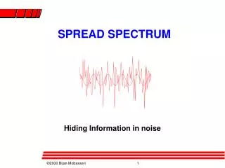
SPREAD SPECTRUM Hiding Information in noise
Origins of Spread Spectrum • Military communication has always been concerned with the following two issues • Security • Jam resistance • In civilian communications, above issues take on different interpretations • privacy • unintentional interference
Spread Spectrum:Data Hiding • Spread spectrum is in effect a way to “hide” information • Useful information is buried in noise. To an eavesdropper, the intercepted message looks juts like noise • The intended receive however is able to recover the information from noise using a special “key”
Types of Spread Spectrum • There are two main types of spread spectrum • Direct Sequence(DS) • Frequency Hopping(FH) • in DS/SS, digital data is multiplied by another bitstream running several hundred times faster • In FH/SS, carrier frequency, normally fixed, jumps around in a “random” manner known only to the intended receive
Direct Sequence • Take the baseband digital data b(t) and modulate it by a “random” bit pattern c(t). The resulting bitstream is m(t)=c(t)b(t) b(t) Tb Tc c(t)
Notations • There are a number of important parameters in SS • b(t): data sequence • c(t): spreading sequence • Tb: bit length • Tc: chip length • N=Tb/Tc: number of chips per bit • N=3 in this figure b(t) Tb c(t) Tc
Communications model: Jamming • The classic jamming model is shown below. we will demonstrate that an SS signal provides superior protection against intentional jamming m(t) b(t) r(t) X c(t) i(t) interference
Spreading Code: PN Sequences • Clearly, randomness is at the heart of spread spectrum • However, if truly random codes are used to spread the signal, receiver would never be able to recover the information • Therefore, we need a “pseudo” random noise known as PN sequences. Pseudo because if you wait long enough, they will repeat
Main Features of PN Sequences • To a casual observer, a PN sequence looks like a random alternations of +/-1. • In truth, however, a PN sequence repeats. Can you spot the period here? • The key to “cracking” the code is to find where the period ends
Where is the “spread”? • It is said that spread spectrum signal looks like random noise to all others but why? • Consider this
PN sequence Generation • PN sequences can be generated by a set of flip-flops with appropriate taps + 1 0 0 So S1 S2 output Initial state: 100 1 0 0 1 1 0 1 1 1 0 1 1 1 0 1 0 1 0 0 0 1 1 0 0 output: 0 0 1 1 1 0 1 0
m-sequences • The preceding sequence repeats itself with a period of 23-1=7 • In general, for an m-stage shift register, the period is at most • If the period is equal to the above, we have maximal lengthor m-sequences
Properties • # of 1’s are always one more than the number of 0’s • Period: 2m-1 • Very desirable (tight) correlation • More on this next
Autocorrelation of m-sequences • Let c(t) be an m-sequence. Its autocorrelation function is given by Tb Shifted by <Tc
Behavior of autocorrelation • The significant property of correlation here is that it can discriminate against the slightest shifts. In fact, shift of just a single chip drops the function by a factor of N Rc() 1 -1/N
How to pick an m-sequence? • Once you pick a length N, the question is how do we generate an m-sequence? • N, fixes the number of shift register stages but you can connect them in many ways • Only a few connections give you valid m-sequences(see Table 9.1 and Figure 9.4) + + + 1 2 3 4 5 N=25-1=31, taps at [5,4,2,1]
Example • A PN sequence is generated using a feedback shift register of length 4. The chip rate is 107 pulses per second. Find • a):PN sequence length • b): Chip duration • c):PN sequence period • Answers • a): if an m-sequence, period is 24-1=15. Less if not • b): 1/107=10-7 sec • c):T=NTc=15x10-7 sec
Processing Gain • Probably the single most important component of an SS system is a quantity called processing gain(PG) • PG is defined by PG=N=Tb/Tc • In other words PGis given by the number of chips within a bit
General Rule • Bandwidth spreads by a factor equal to the processing gain spread bandwidth Wss=(Tb/Tc)W=PGxW
Bandwidth of an SS signal: example • Want to know the bandwidth of a digital signal running at 28.8 Kb/secafter spreading • Consider a m=19 stage shift register • PN sequence period N=219-1~219 • There are 219 chips inside a bit, i.e. Tb=NTc • Therefore, Rc=1/Tc=N/Tb=219x 28.8 Kb/sec • Since bandwidth is proportional to bitrate, the new bandwidth is now 219 or 57 dB higher than the unspread signal
Communications model: Jamming • The classic jamming model is shown below. we will demonstrate that an SS signal provides superior protection against intentional jamming m(t) b(t) r(t) X c(t) i(t) interference
Jamming Scenario • A jammer or interference i(t) tries to interfere with a spread spectrum signal • The corrupted spread spectrum signal at the receiver is put through a conventional correlation detector r(t) z(t) c(t) Data pn seq.
Signal+Jammer at the Output • Let’s walk the spread spectrum signal through the receiver interference desired data
Stopping the Jammer • The jammer appears as c(t)*i(t). In other words we have created a spread spectrum signal out of the jammer! • The bandwidth of a SS signal is very large making it look like white noise. Therefore, a lowpass filter integrator) will let the message b(t) through but will stop most of the jammer appearing as c(t)*i(t)
DS/BPSK • So far we have looked at DS/SS in baseband. • For the actual transmission we need to modulate the signal • Spreading can be done either before or after carrier modulation. See Fig. 9.7, 9.8 and 9.9 while listening to this slide
How does SS provide Protection against Jamming? • It can be shown that the SNR at the input and output of correlation detector is given by
Processing Gain • The improvement in SNR is caused by the processing gain, Tb/Tc. This ratio can be several hundreds or thousands • SNR gain can be as high as 1000(30dB)
BER in the Presence of Jamming • A DS/BPSK in Gaussian noise had a BER of • In the presence of jammer(but no noise)
Jammer acts as white noise • Comparison of the two BER expressions • Equivalently, Eb=PTb where P is the average signal power. Then
Jamming Margin • We just saw that processing gain helps counter jamming power • The ratio of jammer power to signal power is called Jamming margin J/P=PG/(Eb/No) • In dB jm=PG-Eb/No
Example • Digital data is running with bit-lengthTb=4.095 ms.This data is spread using a chip length of Tc=1 microsecond using DS/BPSK. What is the jamming margin if the required BER= 10-5.? • In the presence of random noise alone we need Eb/No=10 to achieve BER= 10-5.
Interpretation • The processing gain is Tb/Tc=4095. Plugging these numbers in the JM expression, we get JM |db=10log4095-10log(10)=26.1 dB • We can maintain BER at the desired level even in the presence of a jammer 26dB(400 times) higher than the desired signal
CDMA:spread spectrum at work • Code Division Multiple Access is one of the two competing digital cellular standards (IS-54). The other is TDMA-based IS-136 • In this area, Comcast has adopted IS-136. Bell Atlantic and Sprint PCS have gone the way of CDMA. • These digital services coincide with the AMPS infrastructure
Differences among the three • AMPS is an example of FDMA. Users are on all the time but on different frequency bands • TDMA uses the same 30KHz band of AMPS but services 3 users. Users are on only during their time slot. • In CDMA, there is neither frequency nor time sharing. Everyone is on simultaneously thus taking up the whole spectrum
CDMA Signal Model • In CDMA, kth user’s signal is spread by a PN code ak unique to the subscriber • M users can be on at the same time
How are users separated? • The familiar correlation receiver will do the job X b1 a1 b2 X a2 b3 X a3
Frequency Hopping SS • Transmitter and receiver always operate on a known frequency band. Once found, anyone can listen in • Imagine a scenario where carrier frequency “hops” around in a random pattern • This pattern is known only to the intended receiver thus nobody else can follow the hop
FH/MFSK • One obvious way to implement FH is to use MFSK. • In the conventional MFSK, carrier frequency jumps are controlled by the message • In FH/MFSK, jumps are controlled by a PN sequence
FH Modalities • Slow frequency hopping • Symbol rate Rs of the MFSK signal is an integer multiple of Rh, the hop rate; several symbols are transmitted on each frequency hop three symbols,same carrier freq.
FH Modalities • Fast frequency hopping • The hop rate Rh is an integer multiple of the MFSK symbol rate Rs; the carrier frequency will change several times even before the symbol ends. one symbol
Generating an FH/MFSK Signal • k-bit segments of the PN code drive the synthesizer-->2^k frequencies FH/MFSK M-ary FSK X BPF Freq synthesizer PN code generator
Parameters of the Slow FH • Chip: an individual FH/MFSK tone of shortest duration • In general, Rc=max(Rh,Rs) • For slow FH 1 FH chip Rc=1 per sec Rs=1 per sec Rh=1/3 per sec
Illustrating Slow FH frequency 1/Rs Rs time 1/Rh PN 001 110 011 001 4 FSK tones, 8 hops, PN period 16,
Fast FH • Carrier frequency hops several times within one symbol one symbol
Time-Frequency Plane of Fast FH frequency time symbol 4 MFSK tones, 2 hops per symbol(hop rate=bitrate), 8 possible hops