Download

1 / 61
610 likes | 722 Vues
Lecture 24. Assorted Topics. (We are sneaking up on control). DC motors and their behavior: a state space example. The meaning of exp( A t ). Block diagrams. The inverted pendulum on a cart (introduction). Cruise control. I want to take a brief segue into the subject of dc motors.

E N D
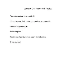
Lecture 24. Assorted Topics (We are sneaking up on control) DC motors and their behavior: a state space example The meaning of exp(At) Block diagrams The inverted pendulum on a cart (introduction) Cruise control
I want to take a brief segue into the subject of dc motors We are going to want to drive and control mechanisms and one way to do that is through motors You can also look at Friedland pp. 18-20
voltage in torque and rotation out
Simple dc motor equations torque rotation rate current back emf We will use, K1 = K = K2 input voltage - back emf = current xresistance (this assumes that i varies slowly enough that inductance is negligible)
We can do a little physics torque = rate of change of angular momentum plug in the motor torque The maximum torque occurs at zero speed The maximum speed occurs at zero torque starting torque no-load speed
Dynamics This is a first order system for the speed You may recall how to solve this in closed form (or you may not)
Note Rewrite Integrate
I left out the initial condition. I can add that in and get the final speed for any voltage. We have Put in a constant of integration Set T = 0 and divide by and we’ll have
If we care about the position of the shaft, not just its speed then we have a second order problem or
This is simpler than the suspension problem we just worked We can look at homogeneous and particular solutions as before We can find the eigenvalues almost by inspection
The eigenvectors are also easy The homogeneous solution
The particular solution can be found by an extension of the first order method recall and recall how we do that retrace those steps using matrices
Note Rewrite Integrate Put in the initial condition
We don’t need to use this fancy method for this problem at the level of what we are used to I’ll address that a bit when we’ve finished this problem Suppose that the input voltage is harmonic in line with the sorts of particular solutions we are used to
Invert Where
Expand Go back to the physical world
Take a look at the initial conditions Here’s the homogeneous solution in its vector form The vector form of the particular solution
Add the two and write the initial condition from which we can find a0 and a1 which I’m not actually going to do today
Note that we can modify all this to get a motor to drive a cart, which we’ll be doing as we go on (remember the overhead crane) force on the cart the motor torque wheel radius The dynamics
The left hand side is stable (its homogeneous solution decays) so a constant voltage leads to a constant speed.
Go back to the weird formula The analysis is outlined in generality in Friedland §3.2, which we will look at later in the course The question that should leap to mind is: What is meant by I don’t want to make too much of this now we’ll tackle it at more length later, but this one is simple enough that we can pursue it a bit
can be defined by the Taylor series We can write our A in the form And write out the first few products
We can combine all of this to write We can recognize these series and write
BLOCK DIAGRAMS The book uses these a lot. I think they can be helpful is understanding how the math works Symbols for multiply, integrate and add We can see how this works by looking at the usual first order system block diagram
second order ode representation state space representation or simple block diagram representation - + a v y -
integrate v to get y “feedback” loops integrate the acceleration to get v - + a u y -
Here are some examples from Friedland one of last year’s texts
translated Friedland’s equations two inputs u two outputs x
The equations for that diagram are dynamics output We won’t be concerned much, if at all, with vector inputs and we won’t deal much with complicated distubances We will not look at systems for which the output depends directly on the input — for us D = 0 Our general systems will look more like
Our control efforts are going to be to find some feedback that will drive an error to zero Let’s take a look at setting up a couple of cases
Inverted pendulum on a cart which problem we will work much later m The errors we want to make vanish will be the angle q some cart position error q l u M y
Energies Constraints The Lagrangian Euler-Lagrange equations
Linearize Solve for the second derivatives Convert to state space
y output B input q output internal “feedback”
I want to start on control at this point We have open loop control and closed loop control Open loop control is simply guess what input u we need to control the system and apply that Closed loop control sits on top of open loop control We measure the error between what we want and what we have and adjust the input to reduce the error: feedback control Recall the diagram from Lecture 1
Ideal output INVERSE PLANT GOAL Mechanical/electromechanical system Actual output + + disturbance input PLANT + - - error feedback CONTROL
About the simplest feedback control system we see in everyday life is cruise control We want to go at a constant speed If the wind doesn’t change and the road is smooth a level we can do this with an open loop system Otherwise we need a closed loop system How does our diagram adapt to this problem?
CRUISE CONTROL the open loop part desired speed INVERSE PLANT GOAL: SPEED nominal fuel flow Actual speed + + PLANT: DRIVE TRAIN Input: fuel flow disturbance - - the closed loop part error Feedback: fuel flow CONTROL
We have some open loop control — a guess as to the fuel flow We have some closed loop control — correct the fuel flow if the speed is wrong It happens that this is not good enough, but let’s just start naively
disturbance simple first order model divide the force open loop part linearize and the goal is to make v’ go to zero
Let’s say a little about possible disturbances hills are probably the easiest to deal with analytically mgsinf f I’ll say more as we go on
The open loop picture + + f v 1/m -