Download
1 / 45
450 likes | 474 Vues
Forecasting is an Integral Part of Business Planning. Inputs: Market, Economic, Other. Demand Estimates. Forecast Method(s). Sales Forecast. Management Team. Business Strategy. Production Resource Forecasts. Examples of Production Resource Forecasts. Forecasting Methods.

E N D
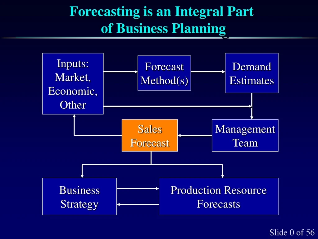
Forecasting is an Integral Part of Business Planning Inputs: Market, Economic, Other Demand Estimates Forecast Method(s) Sales Forecast Management Team Business Strategy Production Resource Forecasts
Forecasting Methods • Qualitative Approaches • Quantitative Approaches
Qualitative Approaches • Usually based on judgments about causal factors that underlie the demand of particular products or services • Do not require a demand history for the product or service, therefore are useful for new products/services • Approaches vary in sophistication from scientifically conducted surveys to intuitive hunches about future events
Qualitative Methods • Executive committee consensus • Delphi method • Survey of sales force • Survey of customers • Historical analogy • Market research
Quantitative Forecasting Approaches • Based on the assumption that the “forces” that generated the past demand will generate the future demand, i.e., history will tend to repeat itself • Analysis of the past demand pattern provides a good basis for forecasting future demand • Majority of quantitative approaches fall in the category of time series analysis
Quantitative Forecasting ApplicationsSmall and Large Firms Source: Nada Sanders and Karl Mandrodt (1994) “Practitioners Continue to Rely on Judgmental Forecasting Methods Instead of Quantitative Methods,” Interfaces, vol. 24, no. 2, pp. 92-100. Note: More than one response was permitted.
Time Series Analysis • A time series is a set of numbers where the order or sequence of the numbers is important, e.g., historical demand • Analysis of the time series identifies patterns • Once the patterns are identified, they can be used to develop a forecast
x x x x x x x x x x x x x x x x x x x x x x x x x x x x x x x x x x x x x x x x x x x x x x Components of Time Series What’s going on here? x Sales 1 2 3 4 Year
Components of Time Series • Trends are noted by an upward or downward sloping line • Seasonality is a data pattern that repeats itself over the period of one year or less • Cycle is a data pattern that repeats itself... may take years • Irregular variations are jumps in the level of the series due to extraordinary events • Random fluctuation from random variation or unexplained causes
Seasonality Length of TimeNumber of Before PatternLength ofSeasons Is RepeatedSeasonin Pattern Year Quarter 4 Year Month 12 Year Week 52 Month Week 4 Month Day 28-31 Week Day 7
Eight Steps to Forecasting • Determining the use of the forecast--what are the objectives? • Select the items to be forecast • Determine the time horizon of the forecast • Select the forecasting model(s) • Collect the data • Validate the forecasting model • Make the forecast • Implement the results
Quantitative Forecasting Approaches • Linear Regression • Simple Moving Average • Weighted Moving Average • Exponential Smoothing (exponentially weighted moving average) • Exponential Smoothing with Trend (double smoothing)
Simple Linear Regression • Relationship between one independent variable, X, and a dependent variable, Y. • Assumed to be linear (a straight line) • Form: Y = a + bX • Y = dependent variable • X = independent variable • a = y-axis intercept • b = slope of regression line
Simple Linear Regression Model • b is similar to the slope. However, since it is calculated with the variability of the data in mind, its formulation is not as straight-forward as our usual notion of slope Yt = a + bx Y 0 1 2 3 4 5 x (weeks)
Regression Equation Example Develop a regression equation to predict sales based on these five points.
Regression Equation Example Slide 18 of 55
Regression Equation Example y = 143.5 + 6.3t 180 175 170 165 Sales 160 155 Forecast Sales 150 145 140 135 Period 1 2 3 4 5 Slide 19 of 55
Forecast Accuracy • Accuracy is the typical criterion for judging the performance of a forecasting approach • Accuracy is how well the forecasted values match the actual values
Monitoring Accuracy • Accuracy of a forecasting approach needs to be monitored to assess the confidence you can have in its forecasts and changes in the market may require reevaluation of the approach • Accuracy can be measured in several ways • Mean absolute deviation (MAD) • Mean squared error (MSE)
Mean Squared Error (MSE) MSE = (Syx)2 Small value for Syx means data points tightly grouped around the line and error range is small. The smaller the standard error the more accurate the forecast. MSE = 1.25(MAD) When the forecast errors are normally distributed
Month Sales Forecast 1 220 n/a 2 250 255 3 210 205 4 300 320 5 325 315 Example--MAD Determine the MAD for the four forecast periods
Month Sales Forecast Abs Error 1 220 n/a 2 250 255 5 3 210 205 5 4 300 320 20 5 325 315 10 40 Solution
Simple Moving Average • An averaging period (AP) is given or selected • The forecast for the next period is the arithmetic average of the AP most recent actual demands • It is called a “simple” average because each period used to compute the average is equally weighted • . . . more
Simple Moving Average • It is called “moving” because as new demand data becomes available, the oldest data is not used • By increasing the AP, the forecast is less responsive to fluctuations in demand (low impulse response) • By decreasing the AP, the forecast is more responsive to fluctuations in demand (high impulse response)
Simple Moving Average • Let’s develop 3-week and 6-week moving average forecasts for demand. • Assume you only have 3 weeks and 6 weeks of actual demand data for the respective forecasts
Simple Moving Average Slide 29 of 55
Simple Moving Average Slide 30 of 55
Weighted Moving Average • This is a variation on the simple moving average where instead of the weights used to compute the average being equal, they are not equal • This allows more recent demand data to have a greater effect on the moving average, therefore the forecast • . . . more
Weighted Moving Average • The weights must add to 1.0 and generally decrease in value with the age of the data • The distribution of the weights determine impulse response of the forecast
Weighted Moving Average Determine the 3-period weighted moving average forecast for period 4 Weights (adding up to 1.0): t-1: .5 t-2: .3 t-3: .2
Exponential Smoothing • The weights used to compute the forecast (moving average) are exponentially distributed • The forecast is the sum of the old forecast and a portion of the forecast error Ft = Ft-1 + a(At-1-Ft-1) • . . . more
Exponential Smoothing • The smoothing constant, , must be between 0.0 and 1.0 (excluding 0.0 and 1.0) • A large provides a high impulse response forecast • A small provides a low impulse response forecast
Exponential Smoothing Example • Determine exponential smoothing forecasts for periods 2 through 10 using =.10 and =.60. • Let F1=D1
Exponential Smoothing Example Slide 38 of 55
Criteria for Selectinga Forecasting Method • Cost • Accuracy • Data available • Time span • Nature of products and services • Impulse response and noise dampening
Reasons for Ineffective Forecasting • Not involving a broad cross section of people • Not recognizing that forecasting is integral to business planning • Not recognizing that forecasts will always be wrong (think in terms of interval rather than point forecasts) • Not forecasting the right things (forecast independent demand only) • Not selecting an appropriate forecasting method (use MAD to evaluate goodness of fit) • Not tracking the accuracy of the forecasting models
How to Monitor andControl a Forecasting Model • Tracking Signal Tracking signal = =
Sources of Forecasting Data • Consumer Confidence Index • Consumer Price Index • Housing Starts • Index of Leading Economic Indicators • Personal Income and Consumption • Producer Price Index • Purchasing Manager’s Index • Retail Sales