Download
1 / 68
690 likes | 870 Vues
Adding Pictures and Shapes to a Worksheet. Lesson 11. Objectives. Software Orientation: The Insert Tab.

E N D
Software Orientation: The Insert Tab • Microsoft Office includes a gallery of images you can insert into worksheets such as pictures, clip art, shapes, and SmartArt graphics. You can also insert a text box that can be positioned anywhere on the worksheet or insert WordArt to call attention to a worksheet or chart’s primary message. Use the Insert tab (see the figure) to insert illustrations and text. • Use this figure as a reference throughout this lesson as you become skilled in inserting and formatting illustrations within a worksheet.
Step-by-Step: Insert a Picture from a File • Before you begin these steps, LAUNCH Microsoft Excel and create a new Blank workbook. • Click the Sheet1 tab. Click Format in the Cells group on the Home tab and click Rename Sheet from the drop-down menu that appears. Key Vernal Fall to replace the selected Sheet1 text, and press Enter. Use the same process to rename Sheet2 to El Capitan and to rename Sheet3 to Sequoias. • Select A1 on the Vernal Fall worksheet. On the Insert tab, click Picture. The Insert Picture dialog box opens.
Step-by-Step: Insert a Picture from a File • In the dialog box directory, navigate to the data files for this lesson, and then click Vernal Fall. Click Insert. The picture is inserted and, as shown in the figure, the Format tab with Picture Tools is added to the Ribbon. • Select the number in the Shape Height text box, key 5, and press Enter. The image changes to a height of 5 inches, with its width automatically proportioned.
Step-by-Step: Insert a Picture from a File • Select A1 on the El Capitan worksheet. Click the Insert tab and click Picture. In the Insert Picture dialog box, navigate to the data files for this lesson and click the El Capitan image, then click Insert. The picture is inserted and the Picture Tools become available. • Select the Shape Height value, key 5, and press Enter. • Select A1 on the Sequoias worksheet. Click the Insert tab and click Picture. In the dialog box, click Sequoias to select it from the data files. Click Insert to insert the picture. • Select the Shape Height value, key 5, and press Enter. • Create a Lesson 11 folder and SAVE as Yosemite. • LEAVE the workbook open to use in the next exercise.
Step-by-Step: Insert a Clip Art Picture • USE the workbook from the previous exercise. • Click on any blank cell in the Sequoia worksheet. On the Home tab, click Insert and click Insert Sheet. Click the rename option in the Cells group, and then click Insert Sheet from the drop-down menu that appears. Click to select the text in the new worksheet’s tab, and then rename the sheet Clip Art. • On the Insert tab, click Clip Art. The Clip Art task pane opens on the right side of the Excel window.
Step-by-Step: Insert a Clip Art Picture • Click the Results should bedrop-down arrow and place a check mark in all media types. In the Searchfor field, key waterfall and click Go. Results are displayed similar to those shown in the figure. • Your results will return more than just graphics. Be sure not to select any audio or video file. Click any image in the search results to insert a waterfall into the Clip Art worksheet.
Step-by-Step: Insert a Clip Art Picture • In the Clip Art task pane, click the arrow in the Resultsshould be field. Deselect all media types except Illustrations (as shown in the figure). Click Go. The results include only clip art images. • Scroll through the list and click an image to insert a waterfall clip art image. • SAVE and CLOSE the workbook. CLOSE the Clip Art task pane. • LEAVE Excel open to use in the next exercise.
Step-by-Step: Use SmartArt Graphics • OPEN the Cruise Dates file for this lesson. • On the Mexico worksheet, select C24. • On the Insert tab, in the Illustrations group, click SmartArt. The Choose a SmartArt Graphicdialog box is displayed as shown in the figure.
Step-by-Step: Use SmartArt Graphics • In the Choose a SmartArt Graphic dialog box, click Cycle in the type pane on the left side of the dialog box. • Click Block Cycle (top row, third from left) in the layout pane on the right side of the dialog box. Click OK. The Cycle graphic image is inserted and SmartArt Tools are available on the Design and Format tabs. When it is inserted, the graphic is joined by its Text pane. This pane allows the user to enter the information to be contained in the SmartArt graphic.
Step-by-Step: Use SmartArt Graphics • On the Design tab, shown in the figure, click the Text Pane button in the Create Graphic group if the Text pane is not displayed when the graphic is inserted. Point to the Block Cycle layout name at the bottom of the Text Pane to see a ScreenTip; holding a description of the best use for the selected SmartArt layout.
Step-by-Step: Use SmartArt Graphics • The Text pane and the SmartArtgraphic have placeholder text that you can replace with your information. The first Text placeholder will be selected as shown in the figure. Key May 20. As you key text in the Text pane, it is displayed in the first block of the Cycle graphic.
Step-by-Step: Use SmartArt Graphics • Click, hold, and drag the SmartArt graphic to rest below the cells in the worksheet. Select E5 in the data range and click Copy. • Click the graphic, select the second [Text] placeholder, and click Paste. The date of June 17 that you copied has now been pasted into the second graphic. • Copy E6 and paste the date in the third [Text] placeholder. • Copy the text in E7 to the fourth [Text] placeholder. • Copy the text in E8 to the last [Text] placeholder. Press Enter to add an additional text placeholder and an additional block to the Cycle graphic.
Step-by-Step: Use SmartArt Graphics • Copy the text in E9 to the last block. • Click outside the image to view the Cycle graphic image as it is displayed in the worksheet. The text pane is hidden from view and only the graphic with its formatting remains. The deselected graphic is shown in the figure. Refer to the previous screen for the graphic with its text pane. • SAVE the workbook as Cruise 1. • LEAVE the workbook open to use in the next exercise.
Step-by-Step: Insert Basic Shapes • USE the workbook from the previous exercise. • On the Alaska worksheet, click A5. Click Shapes in the Illustrations group on the Insert tab. The Shapes gallery shown in the figure opens. • Click Rounded Rectanglein the Rectangles group in the Shapes gallery and click A5 to place the rectangle in that cell. Use the rectangle’s handles to resize it to hide the text in row 5 from A5 to the right boundary of F5 of the worksheet.
Step-by-Step: Insert Basic Shapes • On the Format tab, in the Shape Styles group, click Colored Outline – Orange, Accent 6 (first outline style). This places the colored border around the graphic. • Click Shape Fill in the Shape Styles group and click No Fill. Click an empty cell to deselect the rectangle. The cell’s text is now visible since you chose the no fill option. The colored outline shape calls attention to the Southbound Glacier Discovery cruise that leaves Seattle on June 4. • Click WordArt in the Text group on the Insert tab. In the WordArt gallery, click Fill – Orange, Accent 6 Outline – Accent 6, Glow – Accent 6 (second row, second style). The WordArt sample text Your Text Here is placed.
Step-by-Step: Insert Basic Shapes • Click the Home tab, place your insertion point in the number in the Font Size box and key 36. Press Enter. • The Your text here text is still selected; replace it by keying Lowest Price of the Summer in the WordArt text box. • Move the WordArt text box so that it is several rows directly below the last row of data and aligned with the data range. • On the Insert tab, click Shapes and click Double Arrow (third option from the left) in the Lines group. Click C5 to position the arrow from C5 to the WordArt below the data range (see the figure).
Step-by-Step: Insert Basic Shapes • Click the Insert tab. On the Mexico worksheet, click Shapes. In the Rectangles group, click Snip Same Side Corner Rectangle (fourth from left) in the Rectangles section of the gallery. Click in the center of the existing SmartArt to place the new shape. • Click Colored Outline – Orange, Accent 6 in the Shape Styles group. • Use the shape’s handles to resize the rectangle and drag the rectangle to cover the SmartArt graphic. Click Send Backward in the Arrange group on the Format tab. • SAVE your workbook. • LEAVE the workbook open to use in the next exercise.
Step-by-Step: Draw Lines • USE the workbook from the previous exercise. • On the Advertising worksheet, on the Insert tab, in the Text group, click Text Box. • Select A2 and draw a text box that covers A2:A4. Your cursor will become an upside-down cross when you have chosen the text box option. You simply point to the place where you want to start the box, click, hold, and drag to the area of the worksheet where you want the text box to end and then release the mouse. It might take several tries before you get used to the process (see the figure).
Step-by-Step: Draw Lines • Click inside the box and then key Cruise in the text box. • Click the Insert tab. Click Text Box and select C5. As in step 2, draw a text box that covers C5:C7. • Key Relax in the text box. • Click the Insert tab. Click Text Box and select E8. Draw a text box that covers E8:E10. • Key Enjoy in the text box. • On the Insert tab, click Shapes in the Illustrations group. In the Lines section of the gallery, click Elbow Double-Arrow Connector (sixth from the left). Red circular dots (the connection points) appear on the text boxes as you move your pointer over them.
Step-by-Step: Draw Lines • Click on the Cruise textbox to reveal the connection points. Black indicators show where you can attach a connector. • Click the right connection point on the Cruise text box and drag the connection arrow to the left connection point on the Relax text box. • Use the same procedure in step 8 to connect the Relax text box to the Enjoy text box. Your worksheet should look like the figure.
Step-by-Step: Draw Lines • Click the border of the Cruise text box to display the move arrow. Drag the box to A8. The connection line remains with the text box. • Move the Cruise text box to A2:A4. • SAVE your workbook. • LEAVE the workbook open to use in the next exercise. NOTE: After you have connected the text boxes, you can move the connection line independently, but not the boxes that the connector links.
Step-by-Step: Insert a Block Arrow • USE the workbook from the previous exercise. • On the Hawaii worksheet, click the Insert tab if necessary and then click Shapes. Under Block Arrows, click Right Arrow. • Move the insertion crosshairs to A11 and drag the block so that the arrow point touches the right corner boundary of B12. • The arrow will remain selected. Key Explore the Islands!. • On the Insert tab, click SmartArt, and click Process in the SmartArt type pane.
Step-by-Step: Insert a Block Arrow • Click Continuous Arrow Process (third row, third from left) and click OK. See the figure. • Click any edge of the SmartArt image to display the move pointer and click and drag the pointer to move the image below the block arrow shape.
Step-by-Step: Insert a Block Arrow • The first placeholder is already active. Key Call Today!. • In the second placeholder, key Sail this Summer!. • Select the third [Text] placeholder and press Backspace to delete the third placeholder bullet. • SAVE and CLOSE the workbook. • LEAVE Excel open to use in the next exercise.
Step-by-Step: Create a Flowchart • OPEN the Graphics workbook file for this lesson. • On the Flowchart 1 worksheet, click the Insert tab, and then click Shapes to produce the Shapes gallery. • In the Block Arrows section of the gallery, click Down Arrow. The arrow is now in the work-sheet. Move the newly inserted arrow to the bottom point of the last diamond. Adjust the arrow’s size to resemble the arrows. Move to have the arrow reside below the point of the diamond (see the figure).
Step-by-Step: Create a Flowchart • Click the Insert tab and click Shapes. In the Shapes gallery, click the Flowchart: Process shape. Insert the image below the arrow. Make the newly inserted arrow the approximate size of the existing arrows. • Click in the Process shape, then key Prepare worksheet to calculate potential earnings. • Click Sheet2 and rename it Flowchart 2. • With the Flowchart 2 worksheet the active sheet, click the Insert tab, and click SmartArt. The Choose a SmartArt Graphic dialog box opens.
Step-by-Step: Create a Flowchart • Click Process in the Type pane. Scroll through the list, pointing to the process to locate and click Vertical Process (sixth row, third from left) in the Layout pane. The Vertical Process layout is used to show a progression or sequential steps in a task, process, or work flow from top to bottom. This SmartArt layout works best with Level 1 text without a great deal of detail. Click OK to insert the graphic. The SmartArt Tools tab is now active on the Ribbon. • With the insertion point in the first [Text] placeholder in the Text pane, key Review RFP. • In the second placeholder, key Personnel?.
Step-by-Step: Create a Flowchart • In the third placeholder text box, key Time?. Press Enter. You have now added another text box in the text pane. • Key Prepare Worksheet. The size and shape of the rectangles in the diagram change as you enter a longer text string. • SAVE the workbook as Graphics 1. • LEAVE the workbook open to use in the next exercise.
Step-by-Step: Create an Organization Chart • USE the workbook you saved in the previous exercise. • Click the Sheet3 tab. Right-click, click Format, click Rename Sheet; the Sheet3 text in the worksheet tab is selected. • Key Organization Chart and press Enter. • On the Insert tab, click SmartArt to open the Choose a SmartArt Graphic dialog box. • Click Hierarchy in the Shape Type pane. Click Organization Chart in the layout pane and click OK. • In the first [Text] placeholder, key Margie Shoop, CEO, and press Enter. You have added a new text placeholder.
Step-by-Step: Create an Organization Chart • Click Demote in the Create Graphic group on the Design tab to demote the box to Level 2. This moves the box one level below the CEO and to the left. Key John Y. Chen and press Enter. You have now added another Text placeholder. • Click Demote and key Jamie Reding. Press Enter. This new text placeholder is now one level below John Y. Chen. • Key Stephanie Conway and press Enter. You have now created another text placeholder. • Click Promote and key Ciam Sawyer. Press Enter. You have now created another text placeholder.
Step-by-Step: Create an Organization Chart • Click Demote and key Jeffrey Ford. This now moves the text placeholder one level below Ciam Sawyer. • Click inside the text of the first text placeholder (Margie Shoop, CEO) in the Text pane, then click the drop-down list arrow next to Add Shape in the Create Graphic group on SmartArt Tools Design tab. The Add Shape drop-down list appears. • Click Add Assistant in the drop-down list that appears. Key Brenda Diaz, Assistant in the new text placeholder that appears in Text pane.
Step-by-Step: Create an Organization Chart • Select any blank placeholders in the Text pane and click Delete. If necessary, press Backspace to delete the last blank text placeholder. Move the graphic to the upper left corner of the worksheet. • Click outside the graphic. Your organization chart should look like the figure. • SAVE your workbook. • LEAVE the workbook open to use in the next exercise.
Step-by-Step: Copy or Move a Graphic • USE the workbook you saved in the previous exercise. • Click the Flowchart 2 tab to open the worksheet. • Click the SmartArt graphic to select it. Press the up, down, left, or right directional arrows on your keyboard to move the graphic so that it fills F4:H18. • Click anywhere in the Flowchart 2 graphic. Click Copy on the Home tab to copy the graphic • Click the Flowchart 1 worksheet, select D32, and click Paste; the graphic appears in cell D32.
Step-by-Step: Copy or Move a Graphic • Click the right-center border of the graphic and drag the border to the right boundary of column M. • Click the first rectangle (Review RFP) in the organization chart and drag it to the left and down so that it is parallel to the second rectangle (Personnel?). Notice that the arrow now points to the right towards the other rectangle. • SAVE the workbook. • LEAVE the workbook open to use in the next exercise.
Step-by-Step: Apply Styles to Shapes • USE the workbook from the previous exercise. • On the Flowchart 1 worksheet, at the top of the Organization chart, select the Start shape. The Drawing Tools tab is now active on the Ribbon. • Click the Format tab and click the more arrow next to the predefined Outline Styles in the Shape Styles group. This opens the Outline Colors gallery. • In row 4, click Subtle Effect – Red, Accent 2. You have now applied this style to the Start object.
Step-by-Step: Apply Styles to Shapes • Select the first diamond shape, press Shift, and select the second diamond. You have now selected both objects. • Click Shape Fill and click Red, Accent 2. • With the shapes still selected, click Shape Outline. • Click Dash Dot. • Click Shape Effects, point to Glow, and click the first option (Blue 5 pt. glow, Accent color 1) in the Glow gallery.
Step-by-Step: Apply Styles to Shapes • Click Text Fill in the WordArt Styles group and click Dark Blue in standard colors. You have changed the shape text as illustrated in the figure. • SAVE the workbook. • LEAVE the workbook open to use in the next exercise.
Step-by-Step: Apply Quick Styles to Graphics • USE the workbook from the previous exercise. • On the Flowchart 2 worksheet, select the SmartArt graphic. Click the Design tab. In the SmartArt Styles group, the style that is currently applied to the graphic, based on the Office theme, is selected. The style choices that are available in the SmartArt Styles group on the Design tab are based on the colors, fonts, and effects that comprise the Office theme. • Point to each style that is displayed to see the changes that applying the style would have on the SmartArt graphic. Click White Outline.
Step-by-Step: Apply Quick Styles to Graphics • Click the more arrow in the bottom right corner of Smart Art styles and point to various styles in the Best Match for Document list to observe changes to the graphic. • Preview the styles in the 3-D group and click Metallic Scene (third row, first option on left). When you change the worksheet’s theme, the options in the styles gallery change to reflect the new theme that you have applied to the worksheet.
Step-by-Step: Apply Quick Styles to Graphics • Click Change Colors and click Colorful – Accent Colors. The choices in the SmartArt Styles group have changed based on changing the graphics colors. When you insert a SmartArt graphic, a color diagram of the style you select is displayed on the Choose a SmartArt Graphic dialog box. The color combination displayed in that sample was applied to the graphic when you clicked Change Colors. • On the Organization Chart worksheet, click the SmartArt graphic. Click Subtle Effect in the SmartArt Quick styles window in the SmartArt Styles group. • SAVE the workbook as Graphics 2. • LEAVE the workbook open to use in the next exercise.
Step-by-Step: Resize a Graphic • USE the workbook from the previous exercise. • On the Organization Chart worksheet, click in the SmartArt graphic to select it. • Click the left-center sizing handle and drag it to the column G right boundary. • On the Format tab, click Size. In the Height box, key 5.5. In the Width box, key 6. You have now resized the shape. • Click the shape at the top of the diagram (Margie Shoop, CEO). Click the right sizing handle and drag to the right until the shape extends over the rest of the chart. • SAVE and CLOSE the workbook. • LEAVE Excel open to use in the next exercise.
Step-by-Step: Rotate a Graphic • OPEN the Take a Summer Cruise file for this lesson. • On the Hawaii worksheet, select the text in the standard block arrow (Explore the Islands!). Key Pick a Cruise!. • Click the Format tab. In the Arrange group, click Rotate and click FlipHorizontal. The arrow is reversed. The text will remain facing in the original direction. • Click Rotate and click RotateRight90º. The arrow is now pointing up. • Mouse over the graphic, displaying the move pointer, and move it so that the arrow tip is centered in the whitespace in A6.
Step-by-Step: Rotate a Graphic • Click the SmartArt graphic. On the Design tab, click RighttoLeft in the Create Graphics group. The graphic is reversed horizontally. The text also moved in correspondence with the movement of the arrow. • On the Format tab, click Arrange, and then click SelectionPane. On the Selection and Visibility pane, click RightArrow1. • On the Format tab, click Rotate and then click MoreRotationOptions. The Format Shape dialog box is displayed with the Size options showing. • On the Size and rotate area, click the downarrow in the Rotation field until the graphic rotation is 70º. Click Close.
Step-by-Step: Rotate a Graphic • Move the graphic so that all text is visible and the point is centered in the white space in A6 as illustrated in the figure. • Close the SelectionandVisibility pane. Also, on the Page Layout tab, in the Sheet Options group, deselect the worksheet Gridlines so they no longer display in the worksheet. • SAVE the workbook as Cruise 2. • LEAVE the workbook open to use in the next exercise.
Step-by-Step: Reset a Picture to Its Original State • USE the workbook from the previous exercise. • On the Mexico worksheet, select the picture. The Picture Tools tab is now active. Click the Format tab. • Click the Crop icon. On the drop-down list, click Crop to Shape and then in the Rectangles options, choose Snip Same Side Corner Rectangle. This crops the right and left top corners of the picture.
Step-by-Step: Reset a Picture to Its Original State • In the Picture Quick Styles window, in Picture Styles group, click Metal Frame (3rd style). The corners of the picture have now reappeared and there is a metal frame border in place. • Click the Corrections button in the Adjust group the corrections drop-down list opens. In the Brightness and Contrast area, click Brightness: +20% Contrast: –40% (4th option in first row). You have now adjusted the brightness and contrast of the picture.
Step-by-Step: Reset a Picture to Its Original State • In the Adjust group, click the Color button. The Color drop-down list opens. On the list, in the Recolor section, click Dark Blue, Text color 2 Dark. You have now changed the image to reflect the applied colors (see the figure). • Click Reset Picture in the Adjust group. • SAVE the workbook with the same name and CLOSE. • LEAVE Excel open for the next exercise.
Step-by-Step: Change a Graphic with Artistic Effects • Before you begin these steps, LAUNCH Microsoft Excel and create a new Blank workbook. • Click on the Insert tab. Choose the Skyline image from the Lesson 11 folder. The image is now inserted into the worksheet. • Move the image to align with cell B11. • Under Picture tools, on the Format tab, in the Adjust group, click the Artistic Effects button, shown in the figure.