Download

1 / 51
510 likes | 623 Vues
LC Technology. Manufacturing Systems. Quality Management – Pareto Analysis. Pinpoints problems through the identification and separation of the ‘vital few’ problems from the trivial man y. Vilifredo Pareto: concluded that 80% of the problems with any process are due to 20% of the causes.

E N D
LC Technology Manufacturing Systems
Quality Management – Pareto Analysis Pinpoints problems through the identification and separation of the ‘vital few’ problems from the trivial many. Vilifredo Pareto: concluded that 80% of the problems with any process are due to 20% of the causes.
Quality Management – Pareto Analysis Causes of poor soldering
Quality Management – Pareto Analysis Causes of poor soldering – descending order
Quality Management – Pareto Analysis Cumulative plot is made of all of the causes 80% caused by two problems
Statistical Process Control • Statistical procedure to verify quality • Check manufacturing process is working correctly • Inspect and measure manufacturing process • Varying from target – corrective action taken • Prevents poor quality before it occurs
Statistical Process Control • When? Manufacturing large quantities of items • Euro coins • Computers • Cars etc. • Why? • Impractical to measure each item made • Machine/equipment/human error • How? • Measure a small proportion of the produced items (sample) • Use X-bar and R Charts to see if process is in control • Conclude the quality characteristics of the whole process
Normal Distribution Laser machine A – cutting 20mm hole Some measurement < 20mm Some measurements > 20mm Natural occurrence
Normal Distribution • Machine B making same part as machine A • Same distribution • Skewed to right
Normal Distribution • Histogram: • Statistical information • Column width represents a range of sizes • Shape of histogram is proportional to spread of data Results of a survey on the heights of a group of pupils in a large school Column width = 25mm
Normal Distribution Larger survey – population of a town Column width = 10mm • Centered about mean • Characteristic ‘Bell’ shape curve • Number of occurrences reduce as they deviate from the mean
Normal Distribution A very small sample interval approximates a curve as shown
60 50 40 30 20 10 0 Normal Distribution All measurable attributes show a variation Spread of Sizes = Normal Distribution
Normal Distribution • The spread or ‘width’ of the curve has a precise mathematical meaning - Variance • The greater the variance the wider the curve • Definedby a parameter called the standard deviation
Normal Distribution Calculation of standard distribution (sigma) -measured sizes of a sample of parts y1,y2…etc are the measured values of the sample is the average value N is the number of samples taken
(each value – mean average)² + number of values (6.5 - 7.54)² + (8.2 – 7.54)² + (8.5 – 7.54)² + (7.5 – 7.54)² + (7 – 7.54)² 5 Normal Distribution Sharpen 5 pencils to a length of 8 mm Mean average = 7.54 Sigma = SIGMA= 0.73
Normal Distribution • If sigma is known then we know that: • 95% of parts will lie within +/- 2σ of the mean • 99.74% of parts will lie within +/- 3σ of the mean
Control Charts • Used to establish the control limits for a process • Used to monitor the process to show when it is out of control • X-bar Chart (Mean Charts) • R Charts (Range Charts)
Control Charts Process Mean = Mean of Sample Means Upper control limit (UCL) = Process mean+3 sigma Lower control limit (LCL) = Process mean-3 sigma
Control Charts – X-bar Charts 1. Record measurements from a number of samples sets (4 or 5)
Control Charts – X-bar Charts 2. Calculate the mean of each sample set
Control Charts – X-bar Charts 3. Calculate the process mean (mean of sample means)
Control Charts – X-bar Charts • 4. Calculate UCL and LCL • UCL = process mean + 3σsample • LCL = process mean - 3σsample • The standard deviation σsample of the sample means • where n is the sample size (3 temperature readings) • σ = process standard deviation (4.2 degrees) • σsample =
Control Charts – X-bar Charts • 4. Calculate UCL and LCL • UCL = process mean + 3σsample • LCL = process mean - 3σsample • σsample • UCL = 211 + 3(2.42) = 218.27 degrees • LCL = 211 – 3(2.42) = 203.72 degrees
Control Charts – X-bar Charts UCL = 218.27 LCL = 203.72
Control Charts – X-bar Charts Interpreting control charts: Process out of control Last data point is out of control – indicates definite problem to be addressed immediately as defective products are being made.
Control Charts – X-bar Charts Interpreting control charts: Process in control Process still in control but there is a steady increase toward the UCL. There may be a possible problem and it should be investigated.
Control Charts – X-bar Charts Interpreting control charts: Process in control All data points are all above the process mean. This suggests some non-random influence on the process that should be investigated.
Control Charts – Range Charts The range is the difference between the largest and smallest values in a sample. Range is used to measure the process variation 1. Record measurements from a set of samples
Control Charts – Range Charts 2. Calculate the range = highest – lowest reading
Control Charts – Range Charts 3. Calculate UCL and LCL UCL = D4 x Raverage LCL = D3 xRaverage UCL = 2.57 x 13 = 33.41 degrees LCL = 0 x 13 = 0 degrees
Control Charts – Range Charts UCL R average LCL
Process Capability • Matches the natural variation in a process to the size requirements (tolerance) imposed by the design • Filling a box with washers: • exact number not in all boxes • upper limit set • lower limit set
Process Not Capable Process not capable: a lot of boxes will be over and under filled Normal distribution > specifications Cannot achieve tolerances all of the time
Process Capable Process capable: However there will still be a small number of defective parts Normal distribution is similar to specifications Tolerances will be met most of the time
Process Capable Process capable: No defective parts Normal distribution < specifications Tolerances will be met all the time
Process Capability Index • If Cp =1 • Process is capable • i.e. 99.97% of the natural variation of the process will be within the acceptable limits
Process Capability Index • If Cp > 1 • Process is capable. • i.e. very few defects will be found – less than three per thousand, often much less
Process Capability Index • If Cp <1 • Process is NOT capable • i.e. the natural variation in the process will cause outputs that are outside the acceptable limits.
Statistical Process Control Is doing things right 99% of the time good enough? 13 major accidents at Heathrow Airport every 2 days 5000 incorrect surgical procedures per week ……………… Pharmaceutical company producing 1 000 000 tablets a week, 99% quality would mean tablets would be defective! 10 000 Process of maintaining high quality standards is called : Quality Assurance Modern manufacturing companies often aim for a target of only 3 in a million defective parts. The term six sigma is used to describe quality at this level
Sampling • Size of Sample? • Sufficient to allow accurate assessment of process • More – does not improve accuracy • Less – reduced confidence in result
Sampling Size of Sample S = sample size e = acceptable error - as a proportion of std. deviation z = number relating to degree of confidence in the result
Sampling • Example – find mean value for weight of a packet of sugar • with a confidence of 95% • acceptable error of 10% • Weight of packet of sugar = 1000g • Process standard deviation = 10g
Sampling • z = 1.96 from the table • e = 0.1 (i.e.10%) • Therefore the sample size s = (1.96 / 0.1)2 • Therefore s = 384.16 • Sample size = 385
Sampling • Assume mean weight = 1005g • Sigma = 10g • Therefore error = 10g + 10% = 11g • Result: • 95% confident average weight of all packets of sugar
QC, QA and TQM • Quality Control: • emerged during the 1940s and 1950s • increase profit and reduce cost by the inspection of product quality. • inspect components after manufacture • reject or rework any defective components • Disadvantages: • just detects non-conforming products • does not prevent defects happening • wastage of material and time on scrapped and reworked parts inspection process not foolproof • possibility of non-conforming parts being shipped by mistake
QC, QA and TQM • Quality Assurance • Set up a quality system • documented approach to all procedures and processes that affect quality • prevention and inspection is a large part of the process • all aspects of the production process are involved • system accredited using international standards
QC, QA and TQM • Total Quality Management • International competition during the 1980s and 1990s • Everybody in the organisation is involved • Focussed on needs of the customer through teamwork • The aim is ‘zero defect’ production
Just-In-Time Manufacture Modern products – shortened life cycle Manufacturer – pressure for quick response Quick turnaround - hold inventory of stock Holding inventory costs money for storage Inventory items obsolete before use New approach: Just-In-Time Manufacture
Just-In-Time Manufacture • Underlying concept: Eliminate waste. • Minimum amount: • Materials • Parts • Space • Tools • Time • Suppliers are coordinated with manufacturing company.