Download
1 / 47
470 likes | 589 Vues
Thresholding and multiple comparisons. Information for making inferences on activation. Where? Signal location Local maximum – no inference in SPM Could extract peak coordinates and test (e.g., Woods lab, Ploghaus, 1999) How strong? Signal magnitude

E N D
Information for making inferences on activation • Where? Signal location • Local maximum – no inference in SPM • Could extract peak coordinates and test (e.g., Woods lab, Ploghaus, 1999) • How strong? Signal magnitude • Local contrast intensity – Main thing tested in SPM • How large? Spatial extent • Cluster volume – Can get p-values from SPM • Sensitive to blob-defining-threshold • When? Signal timing • No inference in SPM; but see Aguirre 1998; Bellgowan 2003; Miezin et al. 2000, Lindquist & Wager, 2007
Three “levels” of inference • Voxel-level • Most spatially specific, least sensitive • Cluster-level • Less spatially specific, more sensitive • Set-level • No spatial specificity (no locatization) • Can be most sensitive
Voxel-level Inference • Retain voxels above α-level threshold uα • Gives best spatial specificity • The null hyp. at a single voxel can be rejected uα space Significant Voxels No significant Voxels
Cluster-level Inference • Two step-process • Define clusters by arbitrary threshold uclus • Retain clusters larger than α-level threshold kα uclus space Cluster not significant Cluster significant kα kα
Cluster-level Inference • Typically better sensitivity • Worse spatial specificity • The null hyp. of entire cluster is rejected • Only means that one or more voxels in cluster active uclus space Cluster not significant Cluster significant kα kα
uα α Null Distribution of T t P-val Null Distribution of T Hypothesis Testing • Null Hypothesis H0 • Test statistic T • t observed realization of T • α level • Acceptable false positive rate • Level α = P( T>uα | H0) • Threshold uα controls false positive rate at level α • P-value • Assessment of t assuming H0 • P( T > t | H0 ) • Prob. of obtaining stat. as largeor larger in a new experiment • P(Data|Null) not P(Null|Data)
Multiple Comparisons Problem • Which of 100,000 voxels are significant? • Expected false positives for independent tests: • αNtests • α=0.05 : 5,000 false positive voxels • Which of(e.g.)100 clusters are significant? • α=0.05 : 5 false positives clusters • Solution: determine a threshold that controls the false positive rate (α) per map (across all voxels) rather than per voxel
Why correct? • Without multiple comparisons correction, false positive rate in whole-brain analysis is high. • Using typical arbitrary height and extent threshold is too liberal! (e.g., p < .001 and 10 voxels; Forman et al., 1995). • This is because data is spatially smooth, and false positives tend to be “blobs” of many voxels: =0.10 =0.001 =0.01 True signal inside red square, no signal outside. White is “activation” From Wager, Lindquist, & Hernandez, 2009. “Essentials of functional neuroimaging.” In: Handbook of Neuroscience for the Behavioral Sciences Note: All images smoothed with FWHM=12mm
MCP Solutions:Measuring False Positives • Familywise Error Rate (FWER) • False Discovery Rate (FDR)
False Discovery Rate (FDR): Executive summary FDR = Expected proportion of reported positives that are false positives • (We don’t know what the actual number of false positives is, just the expected number.) • Easy to calculate based on p-value map (Benjamini and Hochberg, 1995) • Always more liberal than FWER control • Adaptive threshold: somewhere between uncorrected and FWER, depending on signal • Can claim that most results are likely to be true positives, but not which ones are false
Family-wise Error Rate vs. False Discovery RateIllustration: Noise Signal Signal+Noise
11.3% 11.3% 12.5% 10.8% 11.5% 10.0% 10.7% 11.2% 10.2% 9.5% 6.7% 10.5% 12.2% 8.7% 10.4% 14.9% 9.3% 16.2% 13.8% 14.0% Control of Per Comparison Rate at 10% Percentage of Null Pixels that are False Positives Control of Familywise Error Rate at 10% FWE Occurrence of Familywise Error Control of False Discovery Rate at 10% Percentage of Activated Pixels that are False Positives
FWE MCP Solutions: Bonferroni • For a statistic image T... • Tiith voxel of statistic image T, where i = 1…V • ...use α = αc/V • αc desired FWER level (e.g. 0.05) • α new alpha level to achieve αc corrected • V number of voxels • Example: for p < .05 and V = 1000 tests, use p < .05/1000 = .00005. • Assumes independent tests (voxels) – but voxels are generally positively correlated (images are smooth)! Conservative under correlation Independent: V tests Some dep.: ? tests Total dep.: 1 test Note: most of the time, this is better: αc = 1 - (1-α)^V, α = 1 – (1-αc) ^ (1/V) See Shaffer, Ann. Rev. Psych. 1995
α FWER MCP Solutions: Controlling FWER w/ Max • FWER is the probability of finding any false positive result in the entire brain map • If any voxel is a false positive, the voxel with the max statistic value (lowest p-value) will be a false positive • Can assess the probability that the max stat value under the null hypothesis exceeds the threshold • FWER is the threshold that controls the probability of the max exceeding that threshold at α Distribution of maxima uα Threshold such that the max only exceeds it α% of the time How to get the distribution of maxima? GRF!
Consider statistic image as lattice representation of a continuous random field Use results from continuous random field theory SPM approach:Random fields… lattice representation
FWER MCP Solutions:Random Field Theory • Euler Characteristic χu • Topological Measure • #blobs - #holes • At high thresholds,just counts blobs • FWER = P(Max voxel χu | Ho) = P(One or more blobs | Ho)= P(χu > 1 | Ho)= E(χu| Ho) Threshold Random Field IF No holes IF Never more than 1 blob How high does the threshold need to be? ~p<.001? Suprathreshold Sets
Random Field Intuition • Corrected P-value for voxel value t depends on • Volume of search area • Roughness of data in search area • The t-value in any given voxel tested • Statistic value t increases • Pc decreases (but only for large t) • Search volume increases • Pc increases (more severe MCP) • Roughness increases (Smoothness decreases) • Pc increases (more severe MCP)
1 2 3 4 5 6 7 8 9 10 1 2 3 4 Random Field TheorySmoothness Parameterization • RESELS = Resolution Elements • 1 RESEL = FWHMx x FWHMy x FWHMz • Volume of search region in units of smoothness • Eg: 10 voxels, 2.5 FWHM = 4 RESELS • Beware RESEL misinterpretation • The RESEL count isnot the number of independent tests in image • See Nichols & Hayasaka, 2003, Stat. Meth. in Med. Res. • Do not Bonferroni correct based on resel count.
Estimate distribution of cluster sizes (mean and variance) Mean: Expected Cluster Size Expected supra-threshold volume / expected number of clusters = E(S) / E(L) = E(L) = E(χu), expected Euler characteristic, assuming no holes (high threshold) This provides uncorrected p-values: Chances of getting a blob of >= k voxels under the null hypothesis …which are then corrected: Pc = E(L) Puncorr 5mm FWHM 10mm FWHM 15mm FWHM Random Field TheoryCluster Size Tests
Lattice ImageData Continuous Random Field Random Field Theory Assumptions and Limitations • Sufficient smoothness • FWHM smoothness 3-4× voxel size (Z) • More like ~10× for low-df T images • Smoothness estimation • Estimate is biased when images not sufficiently smooth • Multivariate normality • Virtually impossible to check • Several layers of approximations • Stationarity required for cluster size results • Cluster size results tend to be too lenient in practice!
FWER correctionStatistical Nonparametric Mapping - SnPMThresholding without (m)any assumptions Almost all slides from Tom Nichols
5% Parametric Null Distribution 5% Nonparametric Null Distribution Nonparametric Inference • Parametric methods • Assume distribution ofstatistic under nullhypothesis • Needed to find P-values, u • Nonparametric methods • Use data to find distribution of statisticunder null hypothesis • Any statistic!
Permutation TestToy Example • Data from V1 voxel in visual stim. experiment A: Active, flashing checkerboard B: Baseline, fixation 6 blocks, ABABAB Just consider block averages... • Null hypothesis Ho • No experimental effect, A & B labels arbitrary • Statistic • Mean difference
Permutation TestToy Example • Under Ho • Consider all equivalent relabelings
Permutation TestToy Example • Under Ho • Consider all equivalent relabelings • Compute all possible statistic values
Permutation TestToy Example • Under Ho • Consider all equivalent relabelings • Compute all possible statistic values • Find 95%ile of permutation distribution
Permutation TestToy Example • Under Ho • Consider all equivalent relabelings • Compute all possible statistic values • Find 95%ile of permutation distribution
Permutation TestToy Example • Under Ho • Consider all equivalent relabelings • Compute all possible statistic values • Find 95%ile of permutation distribution -8 -4 0 4 8
Permutation TestStrengths • Requires only assumption of exchangeability: • Under Ho, distribution unperturbed by permutation • Subjects are exchangeable (good for group analysis) • Under Ho, each subject’s A/B labels can be flipped • fMRI scans not exchangeable under Ho (bad for time series analysis/single subject) • Due to temporal autocorrelation
5% Parametric Null Max Distribution 5% Nonparametric Null Max Distribution Controlling FWER: Permutation Test • Parametric methods • Assume distribution ofmax statistic under nullhypothesis • Nonparametric methods • Use data to find distribution of max statisticunder null hypothesis • Again, any max statistic!
RF & Perm adapt to smoothness Perm & Truth close Bonferroni close to truth for low smoothness FWER Correction: Performance summary Nichols and Hayasaka, 2003 19 df FamilywiseErrorThresholds more 9 df
Permutation vs. Bonferroni: Power curves • Bonferroni and SPM’s GRF correction do not account accurately for spatial smoothness with the sample sizes and smoothness values typical in imaging experiments. • Nonparametric tests are more accurate and usually more sensitive. d = 2 d = 2 d = 1 d = 1 d = 0.5 d = 0.5 From Wager, Lindquist, & Hernandez, 2009. “Essentials of functional neuroimaging.” In: Handbook of Neuroscience for the Behavioral Sciences
Performance Summary • Bonferroni • Not adaptive to smoothness • Not so conservative for low smoothness • Random Field • Adaptive • Conservative for low smoothness & df • Permutation • Adaptive (Exact)
MCP Solutions:Measuring False Positives • Familywise Error Rate (FWER) • Familywise Error • Existence of one or more false positives • FWER is probability of familywise error • False Discovery Rate (FDR) • FDR = E(V/R) • R voxels declared active, V falsely so • Realized false discovery rate: V/R
p(i)< (i/V)q Benjamini & HochbergProcedure • Select desired limit q on FDR (e.g., 0.05) • Order p-values, p(1)<p(2)< ... < p(V) • Let r be largest i such that • Reject all hypotheses corresponding top(1), ... , p(r). • Example: • 1000 Voxels, q = .05 • Keep those above P < .05*i/100 JRSS-B (1995)57:289-300 1 p(i) p-value (i/V)q 0 0 1 i/V • Under positive dependence; OK for fMRI
Benjamini & Hochberg:Key Properties • FDR is controlled E(FDP) = q m0/V • Conservative, if large fraction of nulls false • Adaptive • Threshold depends on amount of signal • More signal, More small p-values,More results with only alpha % expected false discoveries • Hard to find signal in small areas, even with low p-values
Conclusions • Must account for multiple comparisons • Otherwise have a fishing expedition • FWER • Very specific, not very sensitive • FDR • Less specific, more sensitive • Adaptive • Good: Power increases w/ amount of signal • Bad: Number of false positives increases too
References • Most of this talk covered in these papers TE Nichols & S Hayasaka, Controlling the Familywise Error Rate in Functional Neuroimaging: A Comparative Review. Statistical Methods in Medical Research, 12(5): 419-446, 2003. TE Nichols & AP Holmes, Nonparametric Permutation Tests for Functional Neuroimaging: A Primer with Examples. Human Brain Mapping, 15:1-25, 2001. CR Genovese, N Lazar & TE Nichols, Thresholding of Statistical Maps in Functional Neuroimaging Using the False Discovery Rate. NeuroImage, 15:870-878, 2002.
Set-level Inference • Count number of blobs c • c depends on by uclus & blob size k threshold • Worst spatial specificity • Only can reject global null hypothesis uclus space k k Here c = 1; only 1 cluster larger than k
Random Field TheoryCluster Size Corrected P-Values • Previous results give uncorrected P-value • Corrected P-value If E(L) is expected number of clusters: • Bonferroni • Correct for expected number of clusters • Corrected Pc = E(L) Puncorr • Poisson Clumping Heuristic (Adler, 1980) • Corrected Pc = 1 - exp( -E(L) Puncorr )