Download
1 / 19
200 likes | 383 Vues
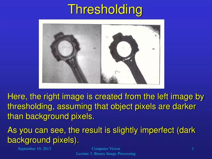
Thresholding. Here, the right image is created from the left image by thresholding, assuming that object pixels are darker than background pixels. As you can see, the result is slightly imperfect (dark background pixels). Geometric Properties.

E N D
Thresholding • Here, the right image is created from the left image by thresholding, assuming that object pixels are darker than background pixels. • As you can see, the result is slightly imperfect (dark background pixels). Computer Vision Lecture 3: Binary Image Processing
Geometric Properties • Let us say that we want to write a program that can recognize different types of tools in binary images. • Then we have the following problem: • The same tool could be shown in different • sizes, • positions, and • orientations. Computer Vision Lecture 3: Binary Image Processing
Geometric Properties Computer Vision Lecture 3: Binary Image Processing
Geometric Properties • We could teach our program what the objects look like at different sizes and orientations, and let the program search all possible positions in the input. • However, that would be a very inefficient and inflexible approach. • Instead, it is much simpler and more efficient to standardize the input before performing object recognition. • We can scale the input object to a given size, center it in the image, and rotate it towards a specific orientation. Computer Vision Lecture 3: Binary Image Processing
Computing Object Size • The size A of an object in a binary image is simply defined as the number of black pixels (“1-pixels”) in the image: A is also called the zeroth-order moment of the object. In order to standardize the size of the object, we expand or shrink the object so that its size matches a predefined value. Computer Vision Lecture 3: Binary Image Processing
Computing Object Position • We compute the position of an object as the center of gravity of the black pixels: These are also called the first-order moments of the object. In order to standardize the position of the object, we shift its position so that it is in the center of the image. Computer Vision Lecture 3: Binary Image Processing
x 1 2 3 4 5 1 2 y 3 4 5 Computing Object Position Compute the center of gravity: • Centering the object within the image: • Binary image: Finally, shift the image content so that the center of gravity coincides with the center of the image. Introduction to Artificial Intelligence Lecture 4: Computer Vision II
Computing Object Orientation • We compute the orientation of an object as the orientation of its greatest elongation. • This axis of elongation is also called the axis of second moment of the object. • It is determined as the axis with the least sum of squared distances between the object points and itself. • In order to standardize the orientation of the object, we rotate it around its center so that its axis of second moment is vertical. Computer Vision Lecture 3: Binary Image Processing
Projections • Projections of a binary image indicate the number of 1-pixels in each column, row, or diagonal in that image. • We refer to them as horizontal, vertical, or diagonal projections, respectively. • Although projections occupy much less memory that the image they were derived from, they still contain essential information about it. Computer Vision Lecture 3: Binary Image Processing
Projections • Knowing only the horizontal or vertical projection of an image, we can still compute the size of the object in that image. • Knowing the horizontal and vertical projections of an image, we can compute the position of the object in that image. • Knowing the horizontal, vertical, and diagonal projections of an image, we can compute the orientation of the object in that image. Computer Vision Lecture 3: Binary Image Processing
Projections Vertical projection Horizontal projection Computer Vision Lecture 3: Binary Image Processing
Projections Diagonal projection Computer Vision Lecture 3: Binary Image Processing
Some Definitions [i-1, j] [i-1, j-1] [i-1, j] [i-1, j+1] • For a pixel [i, j] in an image, … [i, j-1] [i, j] [i, j+1] [i, j-1] [i, j] [i, j+1] [i+1, j] [i+1, j-1] [i+1, j] [i+1, j+1] …these are its 4-neighbors (4-neighborhood). …these are its 8-neighbors (8-neighborhood). Computer Vision Lecture 3: Binary Image Processing
8-path 4-path Some Definitions • A path from the pixel at [i0, j0] to the pixel [in, jn] is a sequence of pixel indices [i0, j0], [i1, j1], …, [in, jn] such that the pixel at [ik, jk] is a neighbor of the pixel at [ik+1, jk+1] for all k with 0 ≤k ≤ n – 1. • If the neighbor relation uses 4-connection, then the path is a 4-path; for 8-connection, the path is an 8-path. Computer Vision Lecture 3: Binary Image Processing
Some Definitions • The set of all 1 pixels in an image is called the foreground and is denoted by S. • A pixel pS is said to be connected to qS if there is a path from p to q consisting entirely of pixels of S. • Connectivity is an equivalence relation, because • Pixel p is connected to itself (reflexivity). • If p is connected to q, then q is connected to p (commutativity). • If p is connected to q and q is connected to r, then p is connected to r (transitivity). Computer Vision Lecture 3: Binary Image Processing
Some Definitions • A set of pixels in which each pixel is connected to all other pixels is called a connected component. • The set of all connected components of –S (the complement of S) that have points on the border of an image is called the background. All other components of –S are called holes. 4-connectedness: 4 objects, 1 hole 8-connectedness: 1 object, no hole To avoid ambiguity, use 4-connectedness for foreground and 8-connectedness for background or vice versa. Computer Vision Lecture 3: Binary Image Processing
original image boundary,interior,surround Some Definitions • The boundary of S is the set of pixels of S that have 4-neighbors in –S. The boundary is denoted by S’. • The interior is the set of pixels of S that are not in its boundary. The interior of S is (S – S’). • Region T surrounds region S (or S is inside T), if any 4-path from any point of S to the border of the picture must intersect T. Computer Vision Lecture 3: Binary Image Processing
1 1 2 2 2 1 1 2 2 3 3 3 3 3 3 3 Component Labeling • Component labeling is one of the most fundamental operations on binary images. • It is used to distinguish different objects in an image, for example, bacteria in microscopic images. • We find all connected components in an image and assign a unique label to all pixels in the same component. Computer Vision Lecture 3: Binary Image Processing
Component Labeling • A simple algorithm for labeling connected components works like this: • Scan the image to find an unlabeled 1-pixel and assign it a new label L. • Recursively assign a label L to all its 1-neighbors. • Stop if there are no more unlabeled 1-pixels. • Go to step 1. • However, this algorithm is very inefficient. • Let us develop a more efficient, non-recursive algorithm. Computer Vision Lecture 3: Binary Image Processing