Download
1 / 17
170 likes | 173 Vues
This study presents blind tests and a unified approach for radar and lidar retrievals in ice clouds. The algorithms accurately retrieve extinction, but IWC and effective radius retrievals are sensitive to mass-size relation. The study also includes simulations of instrumental limitations faced by EarthCARE and assesses the accuracy of retrievals in terms of radiative fluxes and heating rates.

E N D
Radar/lidar retrievals in ice clouds:Blind tests, radiative fluxesand a unified approach Robin Hogan, Malcolm Brooks, Anthony Illingworth University of Reading, UK David Donovan Claire Tinel KNMI, The Netherlands CETP, France
Blind Tests • At the last CloudNet meeting I reported a “Blind Test” of the Donovan and Tinel algorithms: • I used aircraft spectra to simulate radar/lidar profiles • Dave Donovan and Claire Tinel ran their algorithms to derive profiles of extinction, IWC and effective radius • What we found: • Both algorithms retrieved extinction very accurately, even for 1-way optical depths of up to 7 (lidar reduced by 10-6) • Stable to uncertain lidar extinction-to-backscatter ratio • However, re and IWC retrievals sensitive to mass-size relation
In this talk… • Second Blind Test simulates instrumental limitations that will be faced by EarthCARE for: • 10-km dwell (1.4 seconds), 400-km altitude, 355-nm lidar • Instrument noise, finite sensitivity, multiple scattering • Ultimate test: are these retrievals accurate enough to constrain the radiation budget? • Perform radiation calculations on true & measured profiles • Assess errors in terms of fluxes and heating rates • What are the most sensitive of the retrieved parameters? • Radar/lidar combination better than radar alone? • Also test Z-IWC, Z-, Z-re relationships (from EUCREX) • Could the best aspects of the two algorithms be blended into one?
Second Blind Test: more realistic • Ice size distributions from EUCREX aircraft data • Correction for 2D-C undercounting of small ice crystals • Radar • Simulate 100-m oversampling of 400-m Gaussian pulse • Noise added based on signal-to-noise and number of pulses • Lidar • Add molecular scattering appropriate for 355 nm • Instrument noise: photon counting - Poisson statistics • True lidar sensitivity: incomplete penetration of cloud • Multiple scattering: Eloranta model with 20-m footprint • Extinction-to-backscatter unknown but constant with height • Night-time operation, negligible dark current
Radar Instrument noise • Five new profiles from EUCREX dataset • This is what they would look like without instrument noise or multiple scattering • Note strong lidar attenuation Lidar
Radar Instrument noise • Five new profiles… • With instrument noise & multiple scattering • Radar virtually unchanged except finite sensitivity • Lidar noise noticeable • Lidar multiple scattering increases return • Note: “radar-only” relationships derived using same EUCREX dataset so not independent! Lidar
Good case: lidar sees full profile • Extinction and effective radius reasonable when use same habit and include multiple scattering Extinction coefficient Effective radius Donovan: includes multiple scattering Difference between Mitchell and Francis et al. mass-size Tinel: no multiple scattering
Good case: radiation calculations • OLR and albedo good for both radar/lidar and radar-only (but radar-only not independent) Longwave up Mass-size relationship: Error~10 Wm-2 Underestimate radiative effect if multiple scattering neglected Shortwave up
Difference between Mitchell and Francis et al. mass-size relation Wild retrieval where lidar runs out of signal Tinel: no multiple scattering Typical case: radar/lidar retrievals • No retrieval in lower part of cloud • Important to include multiple-scattering in retrieval Extinction coefficient Effective radius Donovan: good retrieval at cloud top
Underestimate radiative effect if multiple scattering neglected Albedo too low (80 W m-2): lower part of cloud is important but mass-size less so (10 W m-2) Typical case: radiative fluxes • At top-of-atmosphere, lower part of cloud important for shortwave but not for longwave OLR excellent:lower part not important Longwave up Shortwave up
Typical profile: Heating rates • Heating profile would be reasonable if full profile was retrieved • What do we do when the lidar runs out of signal? Erroneous 80 K/day heating No cloud observed so no heating by cloud here
Radar/lidar only Blended Scale radar-only retrieval to match here Radar only Possible solution: blend profiles • Where lidar runs out of steam, scale radar-only retrieval for seamless join • Better result than pure radar/lidar or radar only Lidar becomes unreliable here Extinction coefficient Shortwave up
Sensitivity of radiation to retrievals • Longwave: Easy! (for plane-parallel clouds…) • Sensitive to extinction coefficient - good news: this can be retrieved accurately independent of assumption of crystal type • Insensitive to effective radius, habit or extinction/backscatter • OLR insensitive to lower half of cloud undetected by lidar • “Blending” usually gets in-cloud fluxes to better than 5 W m-2 • Shortwave: More difficult • Most sensitive to extinction coefficient • Need full cloud profile: blending enables TOA shortwave to be retrieved to ~10 W m-2, in-cloud fluxes less accurate • Some sensitivity to habit and therefore effective radius • Slight sensitivity to extinction/backscatter ratio • Best way to blend radar/lidar & radar-only profiles?
Differences between algorithms • The two algorithms are the same in their use of radar as a constraint for the lidar inversion, but • Donovan algorithm minimizes Re’ variation in lowest gates • Tinel algorithm minimizes No* variation in whole profile • Multiple scattering currently being added to Tinel algorithm • What are Re’ and No*??? • Basically Re’ ~ (Z/)1/4 • and No* ~ (/Zb)1/(1-b) where b is around 0.42 (from aircraft) • In minimizing variations in these parameters, powers don’t make much difference so • Donovan algorithm minimizes variation in Z/ • Tinel algorithm minimizes variation in Z0.42/ • Now write minimalist version of these algorithms
Unified algorithm? • Minimize variation in which parameter? • Seems more physical that concentration parameter No* is constant? • Better approach: use cost function that penalizes variations in No*, Re’ and extinction (recall wild retrieval earlier) • Minimize variations in furthest gates or in whole profile? • Retrieval much more likely to go wild in furthest gates, so here the constraint should be strongest • Multiple scattering? • Can add Eloranta parameterization in the iterative loop of any algorithm