Download
1 / 40
400 likes | 407 Vues
This chapter explores various methods for determining surface temperature, including slope, three-point, and least squares methods. It also covers water vapor correction and accounting for surface emissivity. The chapter discusses estimating fire size and temperature and issues in remote sensing of surface temperatures.

E N D
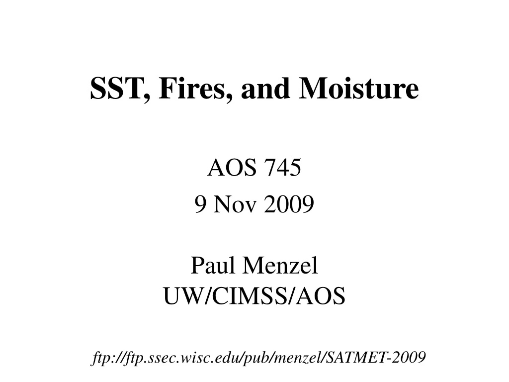
SST, Fires, and Moisture AOS 745 9 Nov 2009Paul MenzelUW/CIMSS/AOS ftp://ftp.ssec.wisc.edu/pub/menzel/SATMET-2009
CHAPTER 7 - SURFACE TEMPERATURE 7.1 Sea Surface Temperature Determination 147 7.1.1 Slope Method 147 7.1.2 Three point Method 148 7.1.3 Least Squares Method 149 7.2. Water Vapor Correction for SST Determinations 149 7.3 Accounting for Surface Emissivity in Determination of SST 152 7.4 Surface Emissivity 153 7.5 Estimating Fire Size and Temperature 154
Issues in Remote Sensing of Surface Temperatures * In IR windows, assuming s ~ 1, in clear skies Tb ~ Tsfc. * The radiometer measures the radiating skin of the surface, hence Tb is not a buoy type temperature measurement. * But window is not free of moisture or aerosol effects, s is not 1, cloud contamination is often difficult to detect. * Much of the activity in the past years has been focussed on addressing these difficulties.
Early algorithms * IRW histogram of occurrence f of observed brightness temperatures T f(T) = fs exp [ -(T - Tsfc)2/22 ] instrument noise / scene variability produce Gaussian distribution; warm side of histogram reveals Ts = T(d2f/dT2=0) - * Three point method combinations of (Ti, fi), (Tj, fj), and (Tk, fk) on the warm side of the histogram enable 3 equations / 3 unknowns, hence a histogram of Ts solutions. * Least squares method ln (f(T)) = ln (fs) - Ts2/22 + TsT/2 - T2/22 has the form ln (f(T)) = Ao + A1T + A2T2 , so Ts = - A1/(2A2) .
Histograms of infrared window brightness temperature in cloud free and cloud contaminated conditions
Water Vapor Correction for SST Determinations * Water vapor correction (T) Ts = Tb + T ranges from 0.1 C in cold/dry to 10 K in warm/moist atmospheres for 11 um IRW observations. * Water vapor correction is highly dependent on wavelength. * Water vapor correction depends on viewing angle. * In IRW for small water vapor concentrations, w = e-Kwu ~ 1 - Kwu so that Ts = Tbw1 + [ Kw1 / (Kw2- Kw1) ] [Tbw1 - Tbw2] . linear extrapolation to moisture free atmosphere was first proposed by Anding and Kauth (1970) * Regression of clear sky IRW obs and collocated buoys create current operational algorithm Ts=A0+A1* Tbw1 +A2*( Tbw1-Tbw2)+A3*(Tbw1-Tbw2)2 a quadratic term helps account for occasional large water vapor concentrations.
Graphic representation of the linear relation between water vapor attenuation and brightness temperature for wet and dry atmospheres
Statistical relations of the water-vapor correction as a function of observed Tb for 3.7 and 11 um spectral channels and 0 and 60 deg viewing angles
Cloud Detection • Several multispectral methods have evolved to detect clouds in the area of interest. • Input data are vis, T3.9, T11, and T12 , T11@30min, • and SST guess. • General tests include: • T11 > 270 K ocean rarely frozen • T11 > T12 + 4 K clouds affect moisture correction • vis < 4% clouds reflect more than ocean sfc • T11 - T3.9 > 1.5 K subpixel clouds • T11 < 0.3 K SST over 1 hr small • -2 K < SST- guess < 5 K SST over days bounded
Weekly AVHRR SST Anomalies for May-June, 1997 show increase in Eastern Equatorial Pacific
1997 El Nino from satellite altimetry (Topex)Sea Level Deviation (cm) wrt 1993-5
Advantages of Geostationary SST Estimates * 10 times more observations of a given location * multispectral cloud detection supplemented by temporal persistence checks * clear sky viewing enhanced by persistence (e.g. can wait for clouds to move through) * daily composite provides good spatial coverage * can discern diurnal excursions in SST * can track SST motions as estimates of ocean currents
David Foley, Joint Institute for Marine and Atmospheric Science, Univ of Hawaii
GOES daily composite SST reveals small scale features in oceans
Sfc Wind Spd 20-22 May 98 xxxxxxxxxxxxxxxxxxxxxx 0 5 10 m/s SSMI sfc wind analysis ((SST) largest where sfc winds < 3 m/s)
Accounting for surface emissivity When the sea surface emissivity is less than one, there are two effects that must be considered: (a) the atmospheric radiation reflects from the surface, and (b) the surface emission is reduced from that of a blackbody. The radiative transfer can be written ps I = B(Ts) (ps) + B(T(p))d(p) o ps + (1-) (ps) B(T(p))d(p) o where (p) represents the transmittance down from the atmosphere to the surface. This can be rewritten I = B(ps)(ps) + B(TA)[1 - (ps) - (ps)2 + (ps)2] . Note that as the atmospheric transmittance approaches unity, the atmospheric contribution expressed by the second term becomes zero.
HIS and GOES radiance observations plotted in accordance with the radiative transfer equation including corrections for atmospheric moisture, non-unit emissivity of the sea surface, and reflection of the atmospheric radiance from the sea surface. Radiances are referenced to 880 cm-1. The intercept of the linear relationship for each data set represents a retrieved surface skin blackbody radiance from which the SST can be retrieved.
Comparison of ocean brightness temperatures measured by a ship borne interferometer (AERI), by an interferometer (HIS) on an aircraft at 20 km altitude, and the geostationary sounder (GOES-8). Corrections for atmospheric absorption of moisture, non-unit emissivity of the sea surface, and reflection of the atmospheric radiance from the sea surface have not been made.
Marine-AERI (Atmospheric Emitted Radiance Interferometer) SST’s measured by 2 AERIs showed mean daily agreement of better than 0.02 K during a cruise from Hawaii to New Zealand
(a) SST error with 1% (sfc) error; (b) (sfc) accuracy needed for SST within 0.3 C Conclusion is you need (sfc) within 0.5% to get SST within 0.3 C.
Stratospheric Aerosol Correction for GOES SST Applying radiative transfer theory to a two-layer model which has water vapor in the troposphere and aerosols in the stratosphere, the measured radiance B(Tb) is (1) where B is Planck function, T is temperature, is transmittance, subscript b, s, t denote brightness, surface, and tropopause, respectively. Using the mean value theorem, Eq. (1) can be written as: (2) where subscripts w and a denote tropospheric water vapor and stratospheric aerosol, respectively.
SST - MODIS and AVHRR MODIS 4 μm Night SST Improved coverage in tropical regions. Color scales are not identical, cloud mask is not applied. AVHRR Night SST
Active Fire Detection Sub-pixel fire causes bigger BT change at 4 um than 11 um (temperature sensitivity) R = p Rfire + (1-p) Rno-fire California – 10/26/03
3.9 and 11.2 microns plotted for one scan line over grassland burning in South America; fires are likely at a, b, and c.
First Order Estimation of TPW Moisture attenuation in atmospheric windows varies linearly with optical depth. - ku = e = 1 - k u For same atmosphere, deviation of brightness temperature from surface temperature is a linear function of absorbing power. Thus moisture corrected SST can inferred by using split window measurements and extrapolating to zero k Ts = Tbw1 + [ kw1 / (kw2- kw1) ] [Tbw1 - Tbw2] . Moisture content of atmosphere inferred from slope of linear relation.
Water vapour evaluated in multiple infrared window channels where absorption is weak, so that w = exp[- kwu] ~ 1 - kwu where w denotes window channel and dw = - kwdu What little absorption exists is due to water vapour, therefore, u is a measure of precipitable water vapour. RTE in window region us Iw = Bsw (1-kwus) + kw Bwdu o us represents total atmospheric column absorption path length due to water vapour, and s denotes surface. Defining an atmospheric mean Planck radiance, then _ _ us us Iw = Bsw (1-kwus) + kwusBw with Bw = Bwdu / du o o Since Bsw is close to both Iw and Bw, first order Taylor expansion about the surface temperature Ts allows us to linearize the RTE with respect to temperature, so _ Tbw = Ts (1-kwus) + kwusTw , where Tw is mean atmospheric temperature corresponding to Bw.
For two window channels (11 and 12um) the following ratio can be determined. _ Ts - Tbw1 kw1us(Ts - Tw1) kw1 _________ = ______________ = ___ _ Ts - Tbw2 kw1us(Ts - Tw2) kw2 where the mean atmospheric temperature measured in the one window region is assumed to be comparable to that measured in the other, Tw1 ~ Tw2, Thus it follows that kw1 Ts = Tbw1 + [Tbw1 - Tbw2] kw2 - kw1 and Tbw - Ts us = . _ kw (Tw - Ts) Obviously, the accuracy of the determination of the total water vapour concentration depends upon the contrast between the surface temperature, Ts, and _ the effective temperature of the atmosphere Tw
MODIS 500 700 T(p) 850