Download
1 / 11
310 likes | 921 Vues
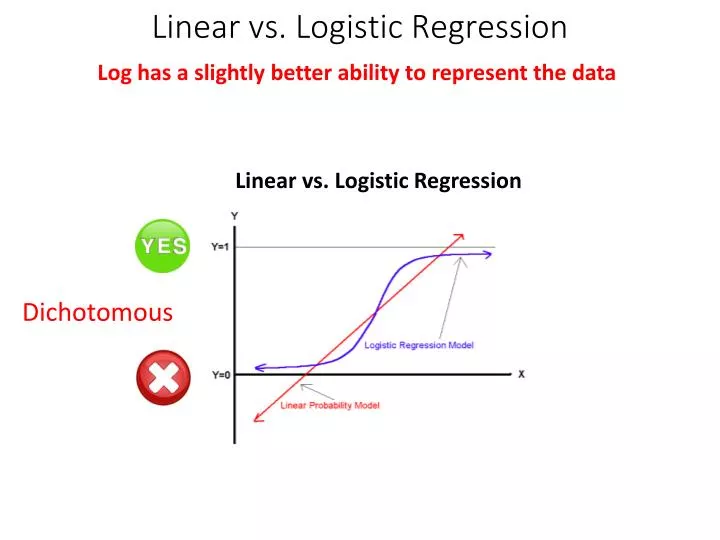
Linear vs. Logistic Regression. Log has a slightly better ability to represent the data. Linear vs. Logistic Regression. Prefer. Dichotomous. Don’t Prefer. History: Logistic Regression. Exponential. Odd’s Ratio.

E N D
Linear vs. Logistic Regression Log has a slightly better ability to represent the data Linear vs. Logistic Regression Prefer Dichotomous Don’t Prefer
History: Logistic Regression Exponential
Odd’s Ratio • Using the values 0 and 1 is helpful for several reasons. Among those reasons is that the values can be interpreted as probabilities
Product of All Probabilities Is Likelihood • Heads or Tails: 50% • Heads twice in a row: 50% * 50% = 25% • The likelihood of purchases by 36 prospects is the product of the probability: • P1 will buy* P2 *. . . * P36
Mathematics Formulas Output Calculations Process `~1:1 Ratio for getting a No or Yes ` The original classification table is put in here to get the Ns as well as to get the original percent among the respondents ln The original percent is turned into a probability Logit Model Includes Log; So Need to Convert to Odds The Regression Beta is then converted to Odds. The Average Odds is then multiplied by the Exp of the Beta. 2.52 vs. 1.03 72% / 28% = 2.6 100%-72% = 28% Delta from the Average Odds Which is then turned back into a percentage Odds = P / (1-P) Odds – (Odds*P) = P Odds = P + Odds*P Odds = P(1 + Odds) P = Odds / (1 + Odds) The original percentage is subtracted from the predicted percent to determine the change
Logistic: Maximum Likelihood • Logistic regression tries out different values for the intercept and the coefficients until it finds the value that results in probabilities—that is, likelihoods —that are closest to the actual, observed probabilities.
Purchase Dataset • Conceptually, if a person has greater income, the probability that he or she will purchase is greater than if the person has less income.
Probability of No Purchase: • Person who did not purchase has a 0 on the Purchased variable • Predicted probability of 2% that he will purchase • Probability of Purchase: • Person who did purchase has a 1 on the Purchased variable • Predicted probability of 94% that this person will purchase • The probabilities are of two different events: • No Purchase and Purchase • In the first case, it’s 98% that he doesn’t purchase, and he doesn’t.
Measure of Goodness • R^2ranges from 0 to 1.0, and can be considered as a percentage of variability. An R 2 of 1.0—or 100%—means that 100% of the variance in the dependent variable can be explained by variability in the independent variable or variables. • We use the log likelihood as our criterion for the “best” coefficients. • The closer to 0.0 a log likelihood: • the better the fit • the closer you’ve come to maximizing the estimate of the likelihood.