Download
1 / 18
180 likes | 312 Vues
Effect of Precipitation Errors on Simulated Hydrological Fluxes and States. Bart Nijssen University of Arizona, Tucson Dennis P. Lettenmaier University of Washington, Seattle. EGS-AGU-EUG Joint Assembly, Nice, France April 11, 2003.

E N D
Effect of Precipitation Errors on Simulated Hydrological Fluxes and States Bart Nijssen University of Arizona, Tucson Dennis P. Lettenmaier University of Washington, Seattle EGS-AGU-EUG Joint Assembly, Nice, France April 11, 2003
Precipitation is the single most important determinant of the fluxes and states of the land surface hydrological system Most important atmospheric input to hydrological models NOAA CPC Summary of the Day 1987-1998 Distribution of surface stations is uneven and sparse in many area Satellite-based precipitation estimates hold great promise for application in hydrological applications Usefulness will depend on error characteristics Motivation
courtesy: NASA GSFC Global Precipitation Measurement Mission • Currently in its formulation phase • Primary spacecraft • Dual-frequency precipitation radar • Passive microwave radiometer • Constellation spacecraft • Passive microwave radiometer • Target launch date: 2007 • Objectives: • Improve ongoing efforts to predict climate • Improve the accuracy of weather and precipitation forecasts • Provide more frequent and complete sampling of the Earth’s precipitation … aims to improve water resources management (NASA/NASDA)
Satellite Precipitation Error • Errors in GPM precipitation products will result from • Instrument error • Algorithm error, e.g. • radar reflectivity - rainfall rate relationships • transfer of information from the primary spacecraft to the constellation spacecraft • Sampling error • result from a lack of temporal continuity in coverage
Objective • To quantify: • the effect of precipitation sampling error on predictions of land surface evapotranspiration, streamflow, and soil moisture at the scale of large continental river basins and tributaries thereof • the variation of the prediction error as a function of the drainage area and the averaging period
Error Model Relative root mean squared error E in time-aggregated precipitation due to sampling error (Steiner, 1996) P - Precipitation (mm/day) A - Domain size (km2) T - Sampling interval (hours) T - Accumulation period (days) • Perturb original precipitation by sampling from a log-normal distribution under the constraints that the corrupted precipitation • is unbiased • has the specified relative error • has the same sequence of wet and dry days A = 2500 km2 T = 1 day Error is uncorrelated in time
Simulated fluxes and states are taken as truth (baseline simulation) Perturb station-based precipitation according to the adopted error model to produce a new time series of precipitation fields • Monte Carlo framework • 5 years • 1000 simulations Rerun the simulations with the new, error-corrupted precipitation Compare newly simulated fluxes and states with the baseline simulation Methodology Simulate the hydrological fluxes and states in a large river basin (Ohio River Basin) using the station-based, gridded precipitation data set from Maurer et al., 2002
Station-based precipitation Maurer et al., 2002 Precipitation (mm) Average precipitation (mm/day) Spatially uncorrelated error Spatially correlated error Perturbation of Precipitation Fields Extract basin precipitation and aggregate to desired resolution (0.5º0.5º) for day X Generate gaussian random fields for each day for each Monte Carlo simulation Corrupt precipitation for day X
Ohio river basin: 5.3105 km2 Mean annual precipitation • Model implementation: • 0.5º0.5º (about 50 km 50 km) • 261 grid cells • Daily timestep Ohio River Basin Streamflow is routed to each red dot along the mainstem of the river (virtual gage locations) Hydrological fluxes and states are averaged over the upstream area associated with each virtual gage location Hydrological fluxes and states are averaged over periods ranging from 1 to 30 days
Analysis: Precipitation • RMSE and bias as a function of area for three sampling intervals • The red dots indicate the virtual gage locations • The dashed lines show the 10% and 90% quantiles
Precipitation • RMSE as a function of averaging period for three upstream areas • (T = 1 hour) • The dashed lines show the 10% and 90% quantiles For the spatially uncorrelated case, precipitation errors decrease rapidly with an increase in averaging period and averaging area
RMSE as a function of area for three sampling intervals RMSE as a function of averaging period for three upstream areas (T = 1 hour) Streamflow Dashed lines show 10% and 90% quantiles Streamflow errors decrease rapidly for areas greater than about 50,000 km2. At the mouth of the Ohio, the relative RMSE in the daily flow was 10-20% for sampling intervals of 1-3 hours
Soil Moisture RMSE as a function of averaging period for three upstream areas (T = 1 hour) Although an increase in the upstream area reduces the mean RMSE, an increase in the averaging period does not reduce the mean RMSE for the deeper soil layers
Spatially Correlated Error RMSE as a function of area for the spatially correlated error (T = 1 hour) The mean RMSE for the uncorrelated error is shown in blue Spatially correlated precipitation errors induce greater persistence in the errors in modeled fluxes when averaged over upstream area
auto correlation function Temporal Correlation in the Error Autocorrelation of the error as a function of the lag for the spatially uncorrelated case for three upstream areas (T = 1 hour) Temporally uncorrelated errors in precipitation give rise to temporally correlated errors in simulated fluxes and states
Conclusions • Errors in precipitation can be large even for hourly overpasses at 50 km resolution. However, the relative errors decrease rapidly for drainage areas larger than about 10,000 km2 • Because of non-linearities in the hydrological cycle, unbiased and temporally uncorrelated errors in precipitation give rise to biases and temporally correlated errors in other fluxes and states • Errors in simulated fluxes and states decline with the averaging area and period. This decrease is less rapid when the errors are temporally and/or spatially correlated • Streamflow errors decrease rapidly for areas greater than about 50,000 km2. At the mouth of the Ohio, the relative RMSE in the daily flow was 10-20% for sampling intervals of 1-3 hours
Manuscript available at: http://www.hydro.washington.edu