Download
1 / 46
460 likes | 675 Vues
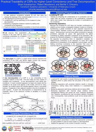
Practical Tractability of CSPs by Higher Level Consistency and Tree Decomposition. Shant Karakashian Dissertation Defense. Collaborations : Bessiere , Geschwender , Hartke , Reeson , Scott, Woodward.

E N D
Practical Tractability of CSPs by Higher Level Consistency and Tree Decomposition ShantKarakashian Dissertation Defense Collaborations: Bessiere, Geschwender, Hartke, Reeson, Scott, Woodward. Support: NSF CAREER Award #0133568 & NSF Grant No. RI-111795. Experiments were conducted on the equipment of the Holland Computing Center at UNL.
Context • Constraint Satisfaction • General paradigm for modeling & solving combinatorial decision problems • Applications in Engineering, Management, Computer Science • Constraint Satisfaction Problems (CSPs) • NP-complete in general • Islands of tractability • Classes of CSPs solvable in polynomial time Karakashian: Ph.D. Defense
Our Focus • One tractabilityconditionlinks [Freuder 82] • Consistency level to • Width of the constraint network, a structural parameter (treewidth) • Catch 22 • Computing width is in NP-hard • Enforcing higher-levels of consistency may require adding constraints, which increases the treewidth • Goal • Exploit above condition to achieve practical tractability Karakashian: Ph.D. Defense
Our Approach • Exploit a tree decomposition • Localize application of the consistency algorithm • Steer constraint propagation along the branches of the tree • Add redundant constraints at separators to enhance propagation • Propose consistency properties that • Enforce a (parameterized) consistency level • While preserving the width of a problem instance Karakashian: Ph.D. Defense
R(*,m)C • Locallization • Bolstering • Sol Counting • Conclusions Background Outline • Background • Contributions • R(∗,m)C: Consistency property & algorithms [SAC 10, AAAI 10] • Localized consistency & structure-guided propagation • Bolstering propagation at separators [CP 12, AAAI 13] • Counting solutions • (Appendices include other incidental contributions) • Conclusions & Future Research Karakashian: Ph.D. Defense
R(*,m)C • Locallization • Bolstering • Sol Counting • Conclusions Background Constraint Satisfaction Problem (CSP) • Given • A set of variables, here X={A,B,C,D,E,F,G} • Their domains, here D={DA,DB,DC,DD,DE,DF,DG}, Di={0,1} • A set of constraints, here C={C1,C2,C3,C4,C5} where Ci= ⟨Ri,scope(Ri)⟩ • Question: Find one solution (NPC), find all solutions (#P) R3 R4 F A E B C D G R1 R2 R5 Karakashian: Ph.D. Defense
R(*,m)C • Locallization • Bolstering • Sol Counting • Conclusions Background Graphical Representations of a CSP D R4 R5 G Hypergraph Primal graph Dual graph R3 A C B F R4 R5 G D R1 R2 E A B R3 C D B,D A,D,G F E R1 B A R2 A,B,C A B A B A,E,F E,B E Karakashian: Ph.D. Defense
R(*,m)C • Locallization • Bolstering • Sol Counting • Conclusions Background Redundant Edges in a Dual Graph • R1R4 forces the value of A in R1 and R4 • The value of A is enforced through R1R3 and R3R4 • R1R4 is redundant R4 R5 D B,D A,D,G B A A B R3 A,B,C A B E A,E,F E,B R1 R2 Karakashian: Ph.D. Defense
R(*,m)C • Locallization • Bolstering • Sol Counting • Conclusions Background Solving CSPs • A CSP can be solved by • Search (conditioning) • Backtrack search • Iterative repair (local search) • Synthesizing & propagating constraints (inference) • Backtrack search • Constructive, exhaustive exploration of search space • Variable ordering improves the performance • Constraint propagation prunes the search tree Karakashian: Ph.D. Defense
R(*,m)C • Locallization • Bolstering • Sol Counting • Conclusions Background Consistency Property: Definition • Example: k-consistency requires that • For all combinations of k-1 variables … all combinations of consistent values … can always be extended to every kth variable • A consistency property • Guarantees that the values of all combinations of variables of a given size verify some set of constraints • Is a necessary but not sufficient condition for partial solution to appear in a complete solution kthvariable any consistent assignment of length k-1 Karakashian: Ph.D. Defense
R(*,m)C • Locallization • Bolstering • Sol Counting • Conclusions Background Algorithms for Enforcing a Consistency Property • May require adding new implicit or redundant constraints • For k-consistency: add constraints to eliminate inconsistent (k-1)-tuples • Which may increase the width of the problem • We propose a consistency property that • Never increases the width of the problem • Allows us to increase & control the level of consistency • Operates by deleting tuples from relations kthvariable any consistent assignment of length k-1 Karakashian: Ph.D. Defense
R(*,m)C • Locallization • Bolstering • Sol Counting • Conclusions Background Tree Decomposition C1 {A,B,C,E} , {R2,R3} C3 C2 {A,E,F},{R1} {A,B,D},{R3,R5} D C4 • Conditions • Each constraint appears in at least one cluster with all the variables in the constraint’s scope • For every variable, the clusters where the variable appears induce a connected subtree • A tree decomposition:〈T, 𝝌, 𝜓〉 • T: a tree of clusters • 𝝌: maps variables to clusters • 𝜓:maps constraints to clusters R4 R5 {A,D,G},{R4} G R3 A C B F R1 R2 E 𝝌(C1) 𝜓(C1) Hypergraph Tree decomposition Karakashian: Ph.D. Defense
R(*,m)C • Locallization • Bolstering • Sol Counting • Conclusions Background Tree Decomposition: Separators • A separator of two adjacent clusters is the set of variables associated to both clusters • Width of a decomposition/network • Treewidth= maximum number of variables in clusters C1 C C1 C2 E {A,B,C,E},{R2,R3} B C3 C3 C2 A F {A,E,F},{R1} {A,B,D},{R3,R5} D C4 C4 G {A,D,G},{R4} Karakashian: Ph.D. Defense
R(*,m)C • Locallization • Bolstering • Sol Counting • Conclusions Background Outline • Background • Contributions • R(∗,m)C: Consistency property & algorithms [SAC 10, AAAI 10] • Localized consistency & structure-guided propagation • Bolstering propagation at separators [CP 12, AAAI 13] • Counting solutions • (Appendices include other incidental contributions) • Conclusions & Future Research Karakashian: Ph.D. Defense
R(*,m)C • Locallization • Bolstering • Sol Counting • Conclusions Background Relational Consistency R(∗,m)C [SAC 2010, AAAI 2010] • A parametrized relational consistency property • Definition • For every set of m constraints • every tuple in a relation can be extended to an assignment • of variables in the scopes of the other m-1 relations • R(*,m)C ≡ every m relations form a minimal CSP Karakashian: Ph.D. Defense
R(*,m)C • Locallization • Bolstering • Sol Counting • Conclusions Background Index-Tree Data Structure • Given: two relations, R1 & R2 • Scope(R1)={X,A,B,C} Scope(R2)={A,B,C,D} • For a given tuple in R1, find matching tuples in R2 Root A 0 1 B 0 1 1 C 1 1 1 t1 t2 t4 t3 Karakashian: Ph.D. Defense
R(*,m)C • Locallization • Bolstering • Sol Counting • Conclusions Background Weakening R(∗,m)C • Weaken R(∗,m)C by removing redundant edges [Jégou 89] R(∗,3)C wR(∗,3)C R1 R2 R3 R1 R2 R4 R1 R2 R5 R1 R3 R4 R2 R3 R4 R2 R4 R5 R3 R4 R5 R1 R2 R3 R1 R2 R5 R1 R3 R4 R2 R4 R5 R3 R4 R5 R1 R2 R1 R2 B B ABD BCF ABD BCF CF CF A CFG CFG C AD AD R5 R5 ADE ACEG ADE ACEG CG CG R3 R4 AE R3 R4 AE Karakashian: Ph.D. Defense
R(*,m)C • Locallization • Bolstering • Sol Counting • Conclusions Background Characterizing R(∗,m)C [Jégou 89] • GAC [Waltz 75] • maxRPWC[Bessiere+ 08] • RmC: Relational m Consistency [Dechter+ 97] R2C R3C R4C RmC R(∗,3)C R(∗,4)C R(∗,m)C R(∗,2)C wR(∗,2)C GAC maxRPWC wR(∗,3)C wR(∗,4)C wR(∗,m)C Karakashian: Ph.D. Defense
R(*,m)C • Locallization • Bolstering • Sol Counting • Conclusions Background Empirical Evaluations (1) Karakashian: Ph.D. Defense
R(*,m)C • Locallization • Bolstering • Sol Counting • Conclusions Background Empirical Evaluations (2) Karakashian: Ph.D. Defense
R(*,m)C • Locallization • Bolstering • Sol Counting • Conclusions Background Algorithms for Enforcing R(∗,m)C • PerTuple • For each tuple find a solution for the variables in the m-1 relations • Many satisfiability searches • Effective when there are many solutions • Each search is quick & easy • AllSol • Find all solutions of problem induced by mrelations, & keep their tuples • A single exhaustive search • Effective when there are few or no solutions • Hybrid Solvers (portfolio based)[+Scott] ti t3 t2 t1 Karakashian: Ph.D. Defense
R(*,m)C • Locallization • Bolstering • Sol Counting • Conclusions Background Hybrid Solver [+Scott] • Choose between PerTuple & AllSol • Parameters to characterize the problem • κpredicts if instance is at the phase transition • relLinkage approximates the likelihood of a tuple at the overlap two relations to appear in a solution • Classifier built using Machine Learning • C4.5 • Random Forests [Gent+ 96] Karakashian: Ph.D. Defense
R(*,m)C • Locallization • Bolstering • Sol Counting • Conclusions Background Decision Tree #1 κ #2 log2(avg(relLinkage)) #3 log2(stDev(relLinkage)) #7 stDev(tupPerVvpNorm) #10 avg(relPerVar) No Yes #1≤ 0.22 Yes No PerTuple #3≤-2.79 Yes No AllSol #7≤0.03 Yes No AllSol #10≤10.05 No Yes PerTuple #2≤-28.75 Yes No #7≤0.23 AllSol AllSol PerTuple Karakashian: Ph.D. Defense
R(*,m)C • Locallization • Bolstering • Sol Counting • Conclusions Background Empirical Evaluations (3) Task: compute the minimal CSP Karakashian: Ph.D. Defense
R(*,m)C • Locallization • Bolstering • Sol Counting • Conclusions Background Outline • Background • Contributions • R(∗,m)C: Consistency property & algorithms [SAC 10, AAAI 10] • Localized consistency & structure-guided propagation • Bolstering propagation at separators [CP 12, AAAI 13] • Counting solutions • (Appendices include other incidental contributions) • Conclusions & Future Research Karakashian: Ph.D. Defense
R(*,m)C • Locallization • Bolstering • Sol Counting • Conclusions Background Localized Consistency • Consistency property cl-R(∗,m)C • Restrict R(∗,m)C to the clusters • Constraint propagation • Guide along a tree structure Karakashian: Ph.D. Defense
R(*,m)C • Locallization • Bolstering • Sol Counting • Conclusions Background Generating a Tree Decomposition • Triangulate the primal graph using min-fill • Identify the maximal cliques using MaxCliques • Connect the clusters using JoinTree • Add constraints to clusters where their scopes appear C1 A,B,C,N C2 A,I,N R5 R7 R1 C3 I,M,N N A B C C4 A,I,K C5 I,J,K R3 D C6 A,K,L R6 I J K C1 C7 B,C,D,H E C7 C {A,B,C,N},{R1} C1 N B,D,F,H C8 C2 M L R2 C8 Elimination order R4 H G F B,D,E,F C3 C9 B D C7 C2 A F,G,H C10 I M C5 K F H C3 C4 C8 C6 L J C4 C5 C6 C10 C9 C10 E G C9 JoinTree min-fill MaxCliques Karakashian: Ph.D. Defense
R(*,m)C • Locallization • Bolstering • Sol Counting • Conclusions Background Information Transfer Between Clusters • Two clusters communicate via their separator • Constraints common to the two clusters • Domains of variables common to the two clusters E R2 R1 R3 R4 A D R4 B A D C B A D C R6 R5 R7 Karakashian: Ph.D. Defense F
R(*,m)C • Locallization • Bolstering • Sol Counting • Conclusions Background Characterizing cl-R(∗,m)C RmC R2C R3C R4C R(∗,3)C R(∗,4)C R(∗,m)C R(∗,2)C ≡ wR(∗,2)C maxRPWC wR(∗,3)C wR(∗,4)C wR(∗,m)C • GAC [Waltz 75] • maxRPWC[Bessiere+ 08] • RmC: Relational m Consistency [Dechter+ 97] GAC cl-R(∗,2)C cl-R(∗,3)C cl-R(∗,4)C cl-R(∗,m)C cl-w(∗,2)C cl-w(∗,3)C cl-w(∗,4)C cl-w(∗,m)C Karakashian: Ph.D. Defense
R(*,m)C • Locallization • Bolstering • Sol Counting • Conclusions Background Empirical Evaluations: Localization Karakashian: Ph.D. Defense
R(*,m)C • Locallization • Bolstering • Sol Counting • Conclusions Background Structure-Guided Propagation • Orderings • Random: FIFO/arbitrary • Static, Priority, Dynamic: Leaves⟷root • Structure-based propagation • Static • Order of MaxCliques • Priority: • Process a cluster once in each direction • Select most significantly filtered cluster • Dynamic • Similar to Priority • But may process ‘active’ clusters more than once C1 A,B,C,N C2 A,I,N Root C3 I,M,N C4 A,I,K C5 I,J,K C6 A,K,L Leaves C1 C7 B,C,D,H {A,B,C,N},{R1} B,D,F,H C8 B,D,E,F C9 C7 C2 F,G,H C10 MaxCliques C3 C4 C8 C5 C6 C10 C9 Karakashian: Ph.D. Defense
R(*,m)C • Locallization • Bolstering • Sol Counting • Conclusions Background Empirical Evaluations: Propagation Karakashian: Ph.D. Defense
R(*,m)C • Locallization • Bolstering • Sol Counting • Conclusions Background Outline • Background • Contributions • R(∗,m)C: Consistency property & algorithms [SAC 10, AAAI 10] • Localized consistency & structure-guided propagation • Bolstering propagation at separators [CP 12, AAAI 13] • Counting solutions • (Appendices include other incidental contributions) • Conclusions & Future Research Karakashian: Ph.D. Defense
R(*,m)C • Locallization • Bolstering • Sol Counting • Conclusions Background Bolstering Propagation at Separators [CP 2012, AAAI 2013] • Localization • Improves performance • Reduces the enforced consistency level • Ideally: add unique constraint • Space overhead, major bottleneck • Enhance propagation by bolstering • Projection of existing constraints • Adding binary constraints • Adding clique constraints E R2 R1 R3 B A D C Rsep R6 R5 R7 F Karakashian: Ph.D. Defense
R(*,m)C • Locallization • Bolstering • Sol Counting • Conclusions Background Bolstering Schemas: Approximate Unique Separator Constraint E Ry R3 D C Ra Rx E E E E E A A D D B B C C R2 R1 R3 A D R2 R1 B C Ry Ra R4 B A D C B A D C B A D C B B A C R3’ R6 R5 R7 R’3 R’3 R6 R5 Rx F F F F F By projection Binary constraints Clique constraints Karakashian: Ph.D. Defense
R(*,m)C • Locallization • Bolstering • Sol Counting • Conclusions Background Resulting Consistency Properties cl+clq-R(∗,2)C cl+clq-R(∗,3)C cl+clq-R(∗,4)C cl+clq-R(∗,|ψ(cli)|)C cl+bin-R(∗,3)C cl+bin-R(∗,4)C cl+bin-R(∗,|ψ(cli)|)C cl+bin-R(∗,2)C cl+proj-R(∗,2)C R(∗,2)C R(∗,4)C cl+proj-R(∗,3)C R(∗,3)C cl+proj-R(∗,4)C cl+proj-R(∗,|ψ(cli)|)C maxRPWC GAC cl-R(∗,2)C cl-R(∗,3)C cl-R(∗,4)C cl-R(∗,|ψ(cli)|)C Karakashian: Ph.D. Defense
R(*,m)C • Locallization • Bolstering • Sol Counting • Conclusions Background Empirical Evaluations Karakashian: Ph.D. Defense
R(*,m)C • Locallization • Bolstering • Sol Counting • Conclusions Background Outline • Background • Contributions • R(∗,m)C: Consistency property & algorithms [SAC 10, AAAI 10] • Localized consistency & structure-guided propagation • Bolstering propagation at separators [CP 12, AAAI 13] • Counting solutions • (Appendices include other incidental contributions) • Conclusions & Future Research Karakashian: Ph.D. Defense
R(*,m)C • Locallization • Bolstering • Sol Counting • Conclusions Background Solution Counting • BTD is used to count the number of solutions [Favier+ 09] • Using Count algorithm on trees [Dechter+ 87] • Witness-based solution counting • Find a witness solution before counting ap Cp wasted no solution Karakashian: Ph.D. Defense
R(*,m)C • Locallization • Bolstering • Sol Counting • Conclusions Background Empirical Evaluations • Task: Count solutions • BTD versus WitnessBTD • GAC: Pre-processing & full look-ahead Karakashian: Ph.D. Defense
R(*,m)C • Locallization • Bolstering • Sol Counting • Conclusions Background Empirical Evaluations Karakashian: Ph.D. Defense
R(*,m)C • Locallization • Bolstering • Sol Counting • Conclusions Background Conclusions • Question • Practical tractability of CSPs exploiting the condition linking • the level of consistency • to the width of the constraint graph • Solution • Introduced a parameterized consistency property R(∗,m)C • Designed algorithms for implementing it • PerTupleand AllSol • Hybrid algorithms • Adapted R(∗,m)C to a tree decomposition of the CSP • Localizing R(∗,m)C to the clusters • Strategies for guiding propagation along the structure • Bolstering separators to strengthen the enforced consistency • Improved the BTD algorithm for solution counting, WitnessBTD • Two incidental results in appendices Karakashian: Ph.D. Defense
R(*,m)C • Locallization • Bolstering • Sol Counting • Conclusions Background Future Research • Extension to non-table constraints • Automating the selection of • a consistency property • consistency algorithms [Geschwender+ 13] • Characterizing performance on randomly generated problems • + much more in dissertation Karakashian: Ph.D. Defense
Thank You Collaborations: Bessiere, Geschwender, Hartke, Reeson, Scott, Woodward. Support: NSF CAREER Award #0133568 & NSF Grant No. RI-111795. Experiments were conducted on the equipment of the Holland Computing Center at UNL. Karakashian: Ph.D. Defense
Computing All k-Connected Subgraphs • Avoids enumerating non-connected k-subgraphs • Competitive on large graphs with small k b a e c d Karakashian: Ph.D. Defense
Solution Cover Problem is in NP-C • Solution Cover Problem • Given a CSPwith global constraints • is there a set of k solutions • such that ever tuple in the minimal CSP is covered by at least one solution in the set? • Set Cover Problem ⟶ Solution Cover Problem • Set Cover Problem • Given a finite set U and a collection S of subsets of U • Are there k elements of S • Whose union is U? Karakashian: Ph.D. Defense