Download
1 / 64
720 likes | 1.09k Vues
Queueing Theory. Chapter 17. Basic Queueing Process. . Arrivals Arrival time distribution Calling population (infinite or finite). Service Number of servers (one or more) Service time distribution. Queue Capacity (infinite or finite) Queueing discipline. “Queueing System”.

E N D
Queueing Theory Chapter 17
Basic Queueing Process • Arrivals • Arrival time distribution • Calling population (infinite or finite) • Service • Number of servers(one or more) • Service time distribution • Queue • Capacity(infinite or finite) • Queueing discipline “Queueing System”
Examples and Applications • Call centers (“help” desks, ordering goods) • Manufacturing • Banks • Telecommunication networks • Internet service • Intelligence gathering • Restaurants • Other examples….
Labeling Convention (Kendall-Lee) ///// Interarrival timedistribution Service timedistribution Number of servers Queueing discipline System capacity Calling population size Notes: FCFS first come, first served LCFS last come, first served SIRO service in random order GD general discipline M Markovian (exponential interarrival times, Poisson number of arrivals) D Deterministic Ek Erlang with shape parameter k G General
Labeling Convention (Kendall-Lee) Examples:M/M/1M/M/5M/G/1M/M/3/LCFSEk/G/2//10M/M/1///100
Terminology and Notation • State of the systemNumber of customers in the queueing system (includes customers in service) • Queue lengthNumber of customers waiting for service = State of the system - number of customers being served • N(t) = State of the system at time t, t ≥ 0 • Pn(t) = Probability that exactly n customers are in the queueing system at time t
Terminology and Notation • n= Mean arrival rate (expected # arrivals per unit time) of new customers when n customers are in the system • s = Number of servers (parallel service channels) • n= Mean service rate for overall system (expected # customers completing service per unit time) when n customers are in the system Note: n represents the combined rate at which all busy servers (those serving customers) achieve service completion.
Terminology and Notation When arrival and service rates are constant for all n, = mean arrival rate (expected # arrivals per unit time) = mean service rate for a busy server 1/ = expected interarrival time 1/ = expected service time = /s= utilization factor for the service facility= expected fraction of time the system’s service capacity (s) is being utilized by arriving customers ()
Terminology and NotationSteady State When the system is in steady state, then Pn = probability that exactly n customers are in the queueing system L = expected number of customers in queueing system = … Lq = expected queue length (excludes customers being served) = …
Terminology and NotationSteady State When the system is in steady state, then = waiting time in system (includes service time) for each individual customer W = E[] q = waiting time in queue (excludes service time) for each individual customer Wq= E[q]
Little’s Formula Demonstrates the relationships between L, W, Lq, and Wq • Assume n= and n= (arrival and service rates constant for alln) • In a steady-state queue, Intuitive Explanation:
Little’s Formula (continued) • This relationship also holds true for (expected arrival rate) when n are not equal. Recall, Pn is the steady state probability of having n customers in the system
Heading toward M/M/s • The most widely studied queueing models are of the form M/M/s (s=1,2,…) • What kind of arrival and service distributions does this model assume? • Reviewing the exponential distribution…. • If T ~ exponential(α), then • A picture of the distribution:
Exponential Distribution Reviewed If T ~ exponential(), then Var(T) = ______ E[T] = ______
Property 1Strictly Decreasing The pdf of exponential, fT(t), is a strictly decreasing function • A picture of the pdf: fT(t) t
Property 2Memoryless The exponential distribution has lack of memory i.e. P(T > t+s | T > s) = P(T > t) for all s, t ≥ 0. Example: P(T > 15 min | T > 5 min) = P(T > 10 min) The probability distribution has no memory of what has alreadyoccurred.
Property 2Memoryless • Prove the memoryless property • Is this assumption reasonable? • For interarrival times • For service times
Property 3Minimum of Exponentials The minimum of several independent exponential random variables has an exponential distribution If T1, T2, …, Tn are independent r.v.s, Ti ~ expon(i) and U = min(T1, T2, …, Tn), U ~expon( ) Example: If there are n servers, each with exponential service times with mean , then U = time until next service completion ~ expon(____)
Property 4Poisson and Exponential If the time between events, Xn ~ expon(), thenthe number of events occurring by time t, N(t) ~ Poisson(t) Note: E[X(t)] = αt, thus the expected number of events per unit time is α
Property 5Proportionality For all positive values of t, and for smallt, P(T ≤ t+t | T > t) ≈ t i.e. the probability of an event in interval t is proportional to the length of that interval
Property 6Aggregation and Disaggregation The process is unaffected by aggregation and disaggregation Aggregation Disaggregation N1 ~ Poisson(1) N1 ~ Poisson(p1) p1 N2 ~ Poisson(2) N2 ~ Poisson(p2) N ~ Poisson() N ~ Poisson() p2 … … pk = 1+2+…+k Nk ~ Poisson(pk) Nk ~ Poisson(k) Note: p1+p2+…+pk=1
Back to Queueing • Remember that N(t), t ≥ 0, describes the state of the system:The number of customers in the queueing system at time t • We wish to analyze the distribution of N(t) in steady state
Birth-and-Death Processes • If the queueing system is M/M/…/…/…/…, N(t) is a birth-and-death process • A birth-and-death process either increases by 1 (birth), or decreases by 1 (death) • General assumptions of birth-and-death processes: 1. Given N(t) = n, the probability distribution of the time remaining until the next birth is exponential with parameter λn 2. Given N(t) = n, the probability distribution of the time remaining until the next death is exponential with parameter μn 3. Only one birth or death can occur at a time
M/M/1 Queueing System • Simplest queueing system based on birth-and-death • We define = mean arrival rate = mean service rate = / = utilization ratio • We require < , that is < 1 in order to have a steady state • Why? Rate Diagram 1 2 3 4 … 0
M/M/1 Queueing System Steady-State Probabilities Calculate Pn, n = 0, 1, 2, …
M/M/1 Queueing System L, Lq, W, Wq Calculate L, Lq, W, Wq
M/M/1 Example: ER • Emergency cases arrive independently at random • Assume arrivals follow a Poisson input process (exponential interarrival times) and that the time spent with the ER doctor is exponentially distributed • Average arrival rate = 1 patient every ½ hour = • Average service time = 20 minutes to treat each patient = • Utilization =
M/M/1 Example: ERQuestions What is the… • probability that the doctor is idle? • probability that there are n patients? • expected number of patients in the ER? • expected number of patients waiting for the doctor? • expected time in the ER? • expected waiting time? • probability that there are at least two patients waiting? • probability that a patient waits more than 30 minutes?
Car Wash Example • Consider the following 3 car washes • Suppose cars arrive according to a Poisson input process and service follows an exponential distribution • Fill in the following table What conclusions can you draw from your results?
M/M/s Queueing System • We define = mean arrival rate = mean service rate s = number of servers (s > 1) = / s = utilization ratio • We require < s , that is < 1 in order to have a steady state Rate Diagram 1 2 3 4 … 0
M/M/s Queueing System Steady-State Probabilities Pn = CnP0 and where
M/M/s Queueing System L, Lq, W, Wq How to find L? W? Wq?
M/M/s Example: A Better ER • As before, we have • Average arrival rate = 1 patient every ½ hour = 2 patients per hour • Average service time = 20 minutes to treat each patient= 3 patients per hour • Now we have 2 doctorss = • Utilization =
M/M/s Example: ERQuestions What is the… • probability that both doctors are idle? • probability that exactly one doctor is idle? • probability that there are n patients? • expected number of patients in the ER? • expected number of patients waiting for a doctor? • expected time in the ER? • expected waiting time? • probability that there are at least two patients waiting? • probability that a patient waits more than 30 minutes?
Travel Agency Example • Suppose customers arrive at a travel agency according to a Poisson input process and service times have an exponential distribution • We are given • = .10/minute = 1 customer every 10 minutes • = .08/minute = 8 customers every 100 minutes • If there were only one server, what would happen? • How many servers would you recommend?
vs. Single Queue vs. Multiple Queues • Would you ever want to keep separate queues for separate servers? Single queue Multiple queues
Bank Example • Suppose we have two tellers at a bank • Compare the single server and multiple server models • Assume = 2, = 3
Bank ExampleContinued • Suppose we now have 3 tellers • Again, compare the two models
M/M/s//K Queueing Model(Finite Queue Variation of M/M/s) • Now suppose the system has a maximum capacity, K • We will still consider s servers • Assuming s ≤ K, the maximum queue capacity is K – s • List some applications for this model: • Draw the rate diagram for this problem:
M/M/s//K Queueing Model(Finite Queue Variation of M/M/s) Rate Diagram Balance equations: Rate In = Rate Out 1 2 3 4 … 0
M/M/s//K Queueing Model(Finite Queue Variation of M/M/s) Solving the balance equations, we get the following steady state probabilities: Verify that these equations match those given in the text for the single server case (M/M/1//K)
M/M/s//K Queueing Model(Finite Queue Variation of M/M/s) To find W and Wq: Although L ≠ lW and Lq ≠ lWq because ln is not equal for all n, where and
M/M/s///N Queueing Model(Finite Calling Population Variation of M/M/s) • Now suppose the calling population is finite • We will still consider s servers • Assuming s ≤ K, the maximum queue capacity is K – s • List some applications for this model: • Draw the rate diagram for this problem:
M/M/s///N Queueing Model(Finite Calling Population Variation of M/M/s) Rate Diagram Balance equations: Rate In = Rate Out 1 2 3 4 … 0