Download
1 / 30
300 likes | 330 Vues
Chapter 22 Cost Curves Key Concept: We define average cost and marginal cost curves and see their connections. c s (y)=c v (y)+F AC s (y) = c s (y)/y = c v (y)/y+F/y = AVC(y)+AFC(y). c s (y)=c v (y)+F MC(y) = ∆ c s (y)/ ∆ y

E N D
Chapter 22 Cost Curves • Key Concept: We define average cost and marginal cost curves and see their connections.
cs(y)=cv(y)+F • ACs(y) = cs(y)/y = cv(y)/y+F/y = AVC(y)+AFC(y)
cs(y)=cv(y)+F • MC(y) = ∆cs(y)/∆y = {[cv(y+∆y)+F]-[cv(y)+F]}/∆y • MVC(y) = ∆cv(y)/∆y = [cv(y+∆y)-cv(y)]/∆y • Thus MC(y)=MVC(y).
All the average costs and marginal costs share the same unit, i.e. dollar/output. • MC(0) = [cv(∆y)-cv(0)]/∆y = cv(∆y)/∆y = AVC(0) • We have seen this before (Ch. 15) at MR(0)=AR(0) or MR at x=0 equals p.
We now explore the relationship between average cost and marginal cost. • Average grade vs. marginal grade
dAVC(y)/dy = d(cv(y)/y)/dy = [yd(cv(y)/dy)-cv(y)]/y2 = [MC(y)-AVC(y)]/y • AVC decreasing MC<AVC • AVC increasing MC>AVC • AVC flat MC=AVC
dAC(y)/dy = d[(cv(y)+F)/y]/dy = [yd((cv(y)+F)/dy)-(cv(y)+F)]/y2 = [MC(y)-AC(y)]/y • AC decreasing MC<AC • AC increasing MC>AC • AC flat MC=AC
MC passes through the minimum of both the AVC and AC. • AVC and AC get closer and y becomes larger because AFC (the difference between AC and AVC) is smaller and smaller.
Since MC(y)=dcv(y)/dy • integrating both sides we get • cv(y)-cv(0)=0yMC(x)dx. • Since cv(0)=0, the area under MC gives you the variable cost. • So there is a connection between the AVC curve and the area under MC curve.
An illustrating example • cv(y)=y2 • cf(y)=1 • AVC(y)=y • AC(y)=y+1/y • MC(y)=2y • minyAC(y) • 1-(1/ y2)=0 y=1
Suppose you have two plants with two different cost functions, what is the cost of producing y units of outputs? • You must use the min cost way. • In interior solution, must allocate y=y1+y2 so that MC1(y1)=MC2(y2). • In other words, the MC of the firm is the horizontal sum.
Similarly if a firm sells to two markets, (in interior solution) must sell to the point where two MRs equal.
Now we turn to the LR. • LR costs: no fixed costs by definition, but AC curve may still be U-shaped because of the quasi-fixed cost. • Quasi-fixed costs are costs that are independent of the level of output, but only need to be paid if the firm produces a positive amount of output.
From above cs(x2(y),y)=c(y) and cs(x2,y)c(y) for all x2. • Hence ACs(x2(y),y)=AC(y) and ACs(x2,y)AC(y) for all x2.
In words, the LR AC is the lower envelope of the SR AC. • This is still true if we have discrete levels of plant size.
Regarding MC • since c(y)=cs(x2(y),y), so MC(y) =dc(y)/dy =cs(x2(y),y)/y+[cs(x2,y)/x2]|x2(y)[x2(y)/y] • Note that x2(y) is defined to be the fixed factor which minimizes the cost, in other words, for a given y, cs(x2,y)/x2=0 at x2=x2(y). So LR MC coincides with SR MC. • Mention discrete levels of plant size.
MC(y) =cs(x2(y),y)/y • LR MC coincides with SR MC. • Let us work out the Cobb Douglas example to convince ourselves.
Chapter 22 Cost Curves • Key Concept: We define average cost and marginal cost curves and see their connections.