Download

1 / 40
460 likes | 1.06k Vues
DEMOGRAPHY. READINGS: FREEMAN, 2005 CHAPTER 52 Pages 1192-1196. What is a Population?. A group of individuals living in a particular area. Individuals that interact while seeking resources and in producing offspring.

E N D
DEMOGRAPHY READINGS:FREEMAN, 2005 CHAPTER 52Pages 1192-1196
What is a Population? • A group of individuals living in a particular area. • Individuals that interact while seeking resources and in producing offspring. • Members of a group that are subject to the same local conditions of the environment. • Members of a single species.
Patterns of Dispersion Individuals in a population may be distributed according to 3 basic patterns of dispersion: * Random * Uniform * Clumped
Random • What? Scattered; no regularity and affinity • Why? Environment uniform; individuals solitary
Uniform • What? About equal distance apart; regular with no affinity • Why? Resource competition; antagonism
Clumped • What? Grouped in some places, absent in others; irregular with affinity • Why? Resources patchy; individuals aggregate
The Frog Problem Dr. T., an ecologist, wanted to find out how many frogs live in a small pond. On the first trip to the pond, 55 frogs were caught, banded, and released. The second trip to the pond, 72 frogs were caught, of those 72 frogs, 12 were banded. Assuming the banded frogs had thoroughly mixed with the unbanded frogs, how many frogs live in the pond?
CAPTURE/RECAPTURE OF FROGS How many frogs in the pond? If X= number of frogs in pond, the proportion of marked frogs on the 1st day must equal the proportion of marked frogs on the 2nd day. X = 72 or X = 55 x 72 = 330 frogs 55 12 12
ABUNDANCE • Most population studies begin with a statement of abundance. • The number of individuals in a population may be obtained by: 1. census- Counting all individuals. 2. sampling- Counting a known fraction to arrive at an estimate of total number. • Many ecological studies require use of sampling, such as capture/recapture or the plot method.
PLOT METHOD OF SAMPLING • Subdivide an area into equal sized plots. • Randomly sample a known proportion of the area. • Calculate the average number of individuals per plot. • Multiply this average times the number of plots in the area.
A Maple Tree Problem A biology student wanted to know how many maple trees there were in his hometown. He knew the town covered an area of 520 blocks. To estimate how many trees, he counted all trees in a random sample of 10 blocks and found that there were 45 maple trees. How many trees are there in his home town?
PLOT METHOD FOR MAPLE TREES How many maple trees in the town? Let X= number of maple trees in town. If a known proportion of equal sized plots are sampled at random, then the number of trees in the area is equal to the average number of trees per plot times the number of plots. X = 45 or X = 520 x 45 = 2340 trees 520 10 10
ACCURACY OF ESTIMATES • Both the capture/recapture and the plot methods are most accurate when distribution of individuals is either uniform or random. Clumped distributions of individuals are highly subject to error. • Larger sample sizes provide the more accurate estimates.
Understanding Check A biologist was concerned about reports that fewer small mouthed bass were being caught in Joe’s Pond. He conducted a capture-recapture study to estimate the size of this fish population. He caught and marked 200 bass and returned them to the pond. The following day, 240 bass were caught of which 60 were marked. When the fish population of any species falls below 500, the pond should be closed to fishing. Should the pond be closed?
POPULATION ECOLOGY • The study of how and why the number of individuals change over time. • Changes in abundance are made through comparison of direct counts or estimates in numbers of individuals. • Changes in density or numbers of individuals per unit area or volume are often used where population sizes are very large or difficult to sample.
MORTALITY, NATALITY AND MOVEMENT • New individuals are added to a population by NATALITY (BIRTHS) or IMMIGRATION (IN MOVEMENT). • Existing individuals are removed from a population by MORTALITY (DEATHS) or EMIGRATION (OUT MOVEMENT).
POPULATION DYNAMICS • If natality (births) and immigration (in movement) exceed mortality (deaths) and emigration (out movement), then populations increase. • If mortality (deaths) and emigration (out movement) exceed natality (births) and immigration (in movement), then populations decrease.
POPULATION DYNAMICS • If natality (births) and immigration (in movement) equals mortality (deaths) and emigration (out movement), then populations are stationary; there is no increase or decrease in number. • Stationary populations are rare, but minor fluctuations around a mean or average population size is common.
A POPULATION DYNAMICS PROBLEM A prairie is inhabited by a ground squirrel population for which: natality is 25 per year mortality is 20 per year immigration is 5 per year emigration is 10 per year This population is: a. increasing. b. decreasing. c. stationary.
DEMOGRAPHY • A study of deaths, births and movements and predictions of how these factors determine the size and structure of populations through time. • Involves construction of life tables, survivorship curves, fecundity tables and calculation of reproductive output.
POPULATION PROJECTIONS Can be made using: 1. Life table, maturnity tables and reproductive outputs. 2. Age structures. 3. Mathematical models that incorporate birth rates, death rates and doubling times.
BASIC DEMOGRAPHIC TOOLS • Life tables are constructed from age specific deaths. lx is the proportion of individuals surviving to a given age. • Age specific fecundity. mx is the number of female births to females of a given age. • Net reproductive output, Ro , is sum lx mx over all age classes.
RO AND POPULATION DYNAMICS The following rules can be used to determine if a population is stationary, increasing or decreasing. The rules are: • If Ro = 1, then population is stationary. • If Ro > 1, then population is growing. • If Ro < 1, then population is declining.
LIFE TABLE • A device for showing mortality changes associated with an age interval (X). • The number of deaths at a given age (DX) is recorded. • The number of survivors at the beginning of an age interval (SX) is determined. • The proportion of “newborns” that survive to a given age interval (lX) is calculated.
AGE SPECIFIC SURVIVORSHIP (lx) • The proportion of live births that survive to the beginning of any age interval is defined as age specific survivorship (lX). • The proportion of the original population alive at age X0 is always 100% or 1.00. Thus, l0 = 1.00 • lX for any subsequent age interval is Sx/S0.
SURVIVORSHIP CURVE • The proportion of individuals living to various ages is the survivorship of a population. • A survivorship curve is constructed by plotting age specific survivorship (lx) and age (X). • Survivorship curves indicate those ages at which mortality is high.
TYPE I SURVIVORSHIP • Some juvenile mortality • Secure middle age • High mortality at old age
TYPE II SURVIVORSHIP • Some to substantial juvenile mortality • Constant mortality thereafter
TYPE III SURVIVORSHIP • Heavy juvenile mortality • Relative security thereafter
A GRAY SQUIRREL POPULATION IN A WOOD LOT • This squirrel population living in an Ohio woodlot has a type II survivorship curve. • Typical of a population with accidental death.
DEMOGRAPHY READINGS:FREEMAN, 2005 CHAPTER 52Pages 1192-1196