Download
1 / 43
440 likes | 550 Vues
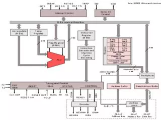
Central Processing Unit Sample Realistic Designs. Major Components of the CPU. Every CPU consists of the three basic components shown in the figure below. Registers hold the inputs of the ALU operations and eventually receive the results.

E N D
Central Processing Unit Sample Realistic Designs
Major Components of the CPU • Every CPU consists of the three basic components shown in the figure below. • Registers hold the inputs of the ALU operations and eventually receive the results. • The control unitcontrols the operationof both ALU andregistersthrough the control signals. • The ALU performs the actualoperations. Registers Control Unit ALU
Realistic Organization • With a large number of registers, dedicated connections are impossible. • Some form of BUS mechanism has to be used to organize the connections. • Most ALU operations require two pieces of data. • We can send them to temporary ALU registers one at a time. • Better yet, we can utilize a two bus system.
Register File Control • Once the results are ready, they have to be sent to the proper register for storage. • The instruction must specify the register and the control unit must enable the right control input. • Registers are usually given a code to reduce the size of the instructions. • This code can be decoded to create the needed load control inputs for the registers.
Controlling the ALU • The ALU is a multi-function unit. • The control unit needs to specify through control signals which operation to be performed. • Putting all of the above together, each microoperation needs the following information: • Select inputs for BUS A. • Select inputs for BUS B • Destination register code. • ALU operation code.
Register Organization Input Data R1 R2 R3 R4 R5 R6 R7 Load Controls S E L B S E L A MUX 1 MUX 2 3 X 8 Decoder Bus B Bus A Arithmetic Logic Unit ALU O P R SELD 3 3 3 5 Control Word SELA SELB SELD OPER
Example of a Microoperation • The control word mentioned above has 14 bits. They will represent the different parts of the microoperations to be performed. • For example, the microoperation: R1 R2 – R3 has the following control word: Field SELA SELB SELD OPER R2 R3 R1 SUB 010 011 001 00101 The control word is 010 011 001 000101
Stack Organization • A useful feature that is included in almost every CPU. • The stack is a storage device that stores information in a Last In First Out (LIFO) manner. • The stack in digital computers is essentially a memory unit with a dedicated address register – the Stack Pointer – that continuously points to the upper most item in the stack. • Items are added to the stack using a PUSH operation and removed from it using a POP. • These operations are simulated through incrementing and decrementing the register.
Register Stack • If the microprocessor has enough registers, it is actually possible to implement the stack operation using registers. • The stack pointer register in this situation would contain the index of the register containing the item at the top of the stack. • With a register stack there would also be a need for a couple of flag registers to determine when the stack is completely full or completely empty.
Stack Based CPUs • There are several CPUs that were designed without general purpose registers. • Instead these CPUs had a fast memory stack that could be used instead of the registers. • In order to effectively use such a system, mathematical expressions have to be re-written in a slightly different manner.
Infix Notation • Common arithmetic expressions are written with the operator between its operands. • This causes a problem for programmers. • Consider the following expression: A * B + C * D • The program must: • Read the entire expression • Extract all of the operands • Extract all of the operations • Decide which operations to do first.
Prefix Notation • It is possible to re-write arithmetic expressions so that the operation is specified before its operands. • This way, there is no need to parse the entire expression. • Read an operation, scan forward until the its two operands are obtained, execute it, continue. • The previous expression can be re-written as: + * A B * C D • We read the + operator first. • Scan forward, we find an * operation. Therefore, the first operand of the + is the result of this *. Perform the * operation. • We find another * operation. Perform it. • Now we have the two operands for the +, perform it.
Reverse Polish Notation • The previous notation is known either as prefix notation or Polish Notation – since it was defined by a Polish mathematician. • A more popular notation is actually the reverse of this one – Reverse Polish Notation (RPN). • Postfix notation. • The operands are specified first, then the operator. • This notation is extremely popular with stack based CPUs. • Like the CPUs in HP’s scientific calculators.
RPN • Our sample expression can be written as: A B * C D * + • It can be evaluated as follows: • Scan from the left, as soon as an operation is found, perform it on the two operands immediately to its left. • Replace the operation and its two operands with the result. • Continue forward.
RPN Evaluation Example • Evaluate the following expression: 1 + 2 * 3 + 4 * 5 * 6 • First, re-write it in RPN: 4 5 * 6 * 2 3 * + 1 + • We find “4 5 *” first. Evaluate that. 20. The expression now becomes: 20 6 * 2 3 * + 1 + • Then we find “20 6 *”. Evaluate it. 120. 120 2 3 * + 1 + • Now we find “2 3 *”. Evaluate it. 6. 120 6 + 1 + • Now we find “120 6 +”. Evaluate it. 126. 126 1 + • Evaluate the last expression “126 1 +”. • The result is 127.
Conversion to RPN • We must follow the hierarchy of operations: • Perform all operations inside inner parenthesis first, then outer ones. • Perform multiplication and division before addition and subtraction. • Example • Translate the following expression to RPN: (A + B) * [C * (D + E) + F] • The result is: A B + D E + C * F + *
Evaluating RPN Expressions with a Stack • Push all operands on the stack until the first operation. • Pop the first two elements off the stack and perform the operation. • Push the result back on the stack. • Continue.
Example • Evaluate the following expression using a stack: 3 4 * 5 6 * + • Push the 3 on the stack. • Push the 4 on the stack. • Pop the 4 and the 3, perform the * operation. • Push the result (12) on the stack. • Push 5 on the stack. • Push 6 on the stack. • Pop the 6 and the 5, perform the * operation. • Push the result (30) on the stack. • Pop the 30 and the 12 off the stack, perform the + operation. • Push the result (42) on the stack.
Example 2 • Evaluate the following expression using a stack: 1 + 2 * 3 + 4 * 5 * 6 • First, re-write it in RPN: 4 5 * 6 * 2 3 * + 1 + 3 5 6 2 2 6 1 4 4 20 20 120 120 120 120 126 126 127 4 5 * 6 * 2 3 * + 1 +
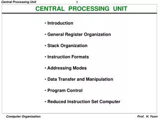
Section 8.8 Reduced Instruction Set Computer (RISC)
Instruction Set vs. Architecture • The design of the instruction set is an important aspect of computer architecture. • The instruction set chosen determines the way machine language programs are constructed. • Early computers had small and simple instruction sets. • Due mainly to the need to reduce the hardware needed to implement them.
CISC - Complex Instruction Set Computers • With the invention of complex ICs, hardware complexity became a non-issue. This lead to the development of some highly complex architectures. • Architectures with instruction sets that contained more than 100 instructions became widely spread. • The trend was to move operations from software to hardware. • Machine instructions like COS, SIN and TAN started to appear. • Actually, some processors also had machine instructions for matrix operations.
RISC - Reduced Instruction Set Computers • Complex instruction sets had a large number of complex instructions. • The complex instructions required a long time to execute. • The instructions required a lot of memory accesses. • Some of the instructions were so specialized that they were used quite infrequently. • In the early 1980s, designers tried to balance that by moving towards simpler instruction sets.
CISC Characteristics • Designers wanted to simplify the process of compilation. • Rather than translate a high level language instruction into many machine language instructions, why not design machine language instructions that implemented them directly. • Complex machine language instructions.
CISC Characteristics • In order to be efficient with memory use, variable length instructions were used. • Register based instructions were short, 1-2 bytes, while memory based instructions were long, up to 5 bytes. • Packing such variable length instructions into a fixed-length memory requires some very special decoding circuits.
CISC Characteristics • Instructions in typical CISC processors provide for direct manipulation of operands in memory. • This will require multiple memory references during the execution of the instruction. • The reason for including these instructions is to simplify the compilation of high-level language programs. • Remember, most variables in a high-level language program are implemented as memory locations. • As more instructions and addressing modes are added to a processor, more logic would be needed to support them. • Ultimately, this leads to a lower performance.
CISC Characteristics in Summary • A large number of instructions. • Typically 100 – 200 instructions. • Some instructions that perform specialized tasks and are used infrequently. • A large variety of addressing modes. • Variable length instruction formats. • Instructions that manipulate operands in memory directly.
RISC Characteristics • RISC tries to reduce execution time by simplifying the instruction set of the computer. • The basic characteristics of RISC processors are: • Relatively few instructions. • Relatively few addressing modes. • Memory access limited to load and store instructions. • All operations are done within the registers of the CPU. • Fixed-length, easily decoded instruction formats. • Single cycle instruction execution. • Hardwired rather than micro-programmed control units.
RISC Characteristics • Mostly register to register operations. • Only simple load and store for memory access. • Operands are read into registers using a load instruction. • The operation is done between the registers. • Results are stored in memory using an explicit store instruction. • This simplifies the instruction set and forces the optimization of register usage. • This also removes the need for many complex addressing modes.
RISC Characteristics • Simple instruction formats. • The instruction length is fixed. • Instructions are aligned to memory words. • Easy to decode instruction formats. • This simplifies the control logic. • Hard-wired control is used to speed-up the generation of control signals.
Single Cycle Instruction Execution • A main feature of RISC processors is their ability to complete the execution of an instruction every clock cycle. • This is done by overlapping the fetch, decode and execute cycles of two or three instructions by using pipelining. • Most CISC processors today also depend on this important feature for speeding up their performance.
Additional Features of RISC Processors • A relatively large number of registers. • This would be useful for storing intermediate results. • Use of overlapped register windows. • This helps speed-up procedure calls. • Compiler support for efficient translation of high-level language programs to make use of these features.
Over-lapped Register Windows • When a function call in a high-level language program requires many operations to implement: • Register values in the calling program must be saved. • Parameters must be placed into appropriate registers for the subroutine. • The subroutine is called. • On the return path, a similar set of operations are needed. • The subroutine has to save its return values in the appropriate registers. • Control is returned to the calling program. • Registers values in the calling program are restored. • All of these are very time consuming.
Over-lapped Register Windows • Given that function calls occur very often in high-level language programs, someway of speeding up this process has to be found. • Some processors use a separate register bank for each procedure. • No need to save and restore the calling procedure’s registers. • RISC processors do a similar thing but it is not dedicated.
Over-lapped Register Windows • Each procedure is allocated a group of registers. • When a function call is being executed, a set of registers are automatically assigned to the new procedure. • Therefore, there is no need to save and restore the calling procedure’s registers. • This new set of registers overlaps by a certain amount with the registers of the calling procedure. • This overlap is used for passing parameters. • When a function is terminated, the registers allocated to it are freed for later use by a different procedure.
Over-lapped Register Window Example R0 • Our CPU has a total of 74 registers. • When a program starts, 10 registers are allocated for global data. • The main program is allocated 10 registers for its local data. • The main program calls function A. • 6 registers are allocated for passing data back and forth between main and A. • 10 registers are allocated to A for local data. • A calls B. • 6 registers are allocated common to A and B. • 10 registers are allocated to B for local data. • Each procedure can access a total of 32 registers. Global Reg. R9 R10 Main Local Reg. R19 R20 Shared Main, A R25 R26 A Local Reg. R35 R36 Shared A, B R41 R42 B Local Reg. R51 R52 Free Reg. R73
Effects on Programming • High level languages – no effect. • All of this is done by the compiler. • Assembly language – registers no longer have a set name. • If you write an instruction of the form: ADD R1, R2 there is no guarantee that you will actually use R1 and R2 of the processor. • The above instruction means, use the first register and the second register in my window.
Over-lapped Window Parameters • The number of registers allocated for each type is a parameter of the processor design. • G the number of global registers. • L the number of local registers. • C the number of common register. all of these depend on the design of the CPU. • In some processor designs, these parameters are decided dynamically. • Depending on the total number of procedures and the total number of registers, a procedure’s window size may change. • The operating system now has to be very intelligent.
32-bit processor. 32-bit address. 8, 16, or 32-bit data. 32-bit instruction format. 31 instructions. 12 Data Manipulation. 11 Data Transfer. 8 Program Control. 3 addressing modes: Register. Immediate. Relative to PC. 138 registers. 10 Global registers. 10 windows of 32 registers each. Berkeley RISC I – Example RISC CPU
Berkeley RISC I • Since only 32 registers are accessible at any point in time, only 5 bits are needed for register selection. • Instructions utilize a three address format. • Destination Register. • Source Register. • Second Source Register or Immediate Data. • Register R0 is a constant 0 all the time. • It can be used to fool the processor into performing additional addressing modes.
Instruction Formats Register Mode Opcode Rd Rs 0 Not Used S2 8 5 5 1 8 5 S2 - Register Register-Immediate Mode Opcode Rd Rs 1 S2 8 5 5 1 13 S2 – Immediate Data PC Relative Mode Opcode Cond Y 8 5 19 Y – Relative Displacement