Download
1 / 26
260 likes | 419 Vues
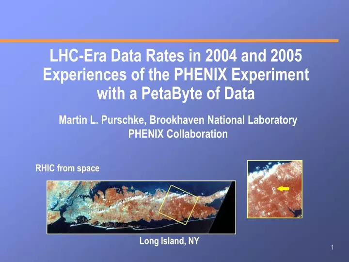
LHC-Era Data Rates in 2004 and 2005 Experiences of the PHENIX Experiment with a PetaByte of Data. Martin L. Purschke, Brookhaven National Laboratory PHENIX Collaboration. RHIC from space. Long Island, NY. RHIC/PHENIX at a glance. PHENIX: 4 spectrometer arms 12 Detector subsystems

E N D
LHC-Era Data Rates in 2004 and 2005Experiences of the PHENIX Experiment with a PetaByte of Data Martin L. Purschke, Brookhaven National Laboratory PHENIX Collaboration RHIC from space Long Island, NY
RHIC/PHENIX at a glance PHENIX: 4 spectrometer arms 12 Detector subsystems 400,000 detector channels Lots of readout electronics Uncompressed Event size typically 240 -170 - 90 KB for AuAu, CuCu, pp Data rate 2.4KHz (CuCu), 5KHz (pp) Front-end data rate 0.5 - 0.9 GB/s Data Logging rate ~300-450MB/s, 600 MB/s max RHIC: 2 independent rings, one beam clockwise, the other counterclockwise sqrt(SNN)= 500GeV * Z/A ~200 GeV for Heavy Ions ~500 GeV for proton-proton (polarized)
Where we are w.r.t. others ALICE ~1250 All in MB/s all approximate 600 ATLAS CMS ~300 LHCb ~150 ~100 ~100 ~25 ~40 400-600MB/s are not so Sci-Fi these days
Outline • What was planned, and what we did • Key technologies • Online data handling • How offline / the users cope with the data volumes Related talks: Danton Yu, “BNL Wide Area Data Transfer for RHIC and ATLAS:Experience and Plan” this (Tuesday) afternoon 16:20 Chris Pinkenburg, “Online monitoring, calibration, and reconstruction in the PHENIX Experiment”, Wednesday 16:40 (OC-6)
A Little History • In its design phase, PHENIX had settled on a “planning” number of 20MB/s data rate (“40 Exabyte tapes, 10 postdocs”) • In Run 2 (2002) we started to approach that 20MB/s number and ran Level-2 triggers • In Run 3 (2003) we faced the decision to either go full steam ahead with Level-2 triggers… or first try something else • Several advances in various technologies conspired to make first 100MB/s, then multi-100MB/s data rates possible • We are currently logging at about 60 times higher rates than the original design called for
But is this a good thing? We had a good amount of discussions about the merit of going to high data rates. Are we drowning in data? Will we be able to analyze the data quickly enough? Are we recording “boring” events, mostly? Is it not better to trigger and reject? • In Heavy-Ion collisions, the rejection power of level2- triggers is limited (high multiplicity, etc) • triggers take a lot of time to study and developers usually welcome a delay in the onset of the actual rejection mode • The rejected events are by no means “boring”, high-statistics physics in them, too
...good thing? Cont’d • Get the data while the getting is good - the Detector system is evolving and is hence unique for each run, better get as much data with it as you can • Get physics that you simply can’t trigger on • Don’t be afraid to let data sit on tape unanalyzed - computing power increases, time is on your side here In the end we convinced ourselves that we could (and should) do it. The increased data rate helped defer the onset of the LVL2 rejection mode in Runs 4, 5 (didn’t run rejection at all in the end) Saved a lot of headaches… we think
Ingredients to achieve the high rates We implemented several main ingredients that made the high rates possible. • We compress the data before they get on a disk the first time (cram as much information as possible into each MB) • Run several local storage servers (“Buffer boxes”) in parallel, and dramatically increased the buffer disk space (40TB currently) • Improved the overall network connectivity and topology • Automated most of the file handling so the data rates in the DAQ become manageable
Event Builder Layout Event Builder Buffer Box Gigabit Crossbar Switch ATP SEB Buffer Box ATP SEB ATP SEB Buffer Box ATP SEB ATP To HPSS SEB Buffer Box ATP SEB ATP SEB Buffer Box ATP SEB ATP SEB Buffer Box ATP SEB Some technical background... The pieces are sent to a given Assembly-and-Trigger Processor (ATP) on a next-available basis, fully assembled event available here for the first time The data are stored on “Buffer boxes” that help ride out the ebb and flow of the data stream, ride out service interruptions of the HPSS tape system, and help send a steady stream to the tape robot Sub-Event buffers see parts of a given Event following the granularity of the Detector electronics With ~50% combined uptime of PHENIX * RHIC, we can log 2x the HPSS max data rate in the DAQ. Just needs enough buffer depth (40TB)
Data Compression This is what a file normally looks like buffer buffer buffer buffer buffer buffer LZO algorithm Add new buffer hdr New buffer with the compressed one as payload This is what a file then looks like On readback: LZO Unpack Original uncompressed buffer restored Found that the raw data are still gzip-compressible after zero-suppression and other data reduction techniques Introduced a compressed raw data format that supports a late-stage compression All this is handled completely in the I/O layer, the higher-level routines just receive a buffer as before.
Breakthrough: Distributed Compression Event Builder Buffer Box Gigabit Crossbar Switch ATP SEB Buffer Box ATP SEB ATP SEB Buffer Box ATP SEB ATP To HPSS SEB Buffer Box ATP SEB ATP SEB Buffer Box ATP SEB ATP SEB Buffer Box ATP SEB The compression is handled in the “Assembly and Trigger Processors” (ATP’s) and can so be distributed over many CPU’s -- that was the breakthrough The Event builder has to cope with the uncompressed data flow, e.g. 500MB/s … 900MB/s The buffer boxes and storage system see the compressed data stream, 250MB/s … 450MB/s
Buffer Boxes • We use COTS dual-CPU machines, some SuperMicro or Tyan MoBo designed for data throughput • SATA 400G disk arrays (16 disks) Sata->SCSIRaid controller in striping (Raid0) mode • 4 1.7 TB systems across 4 disks each on 6 Boxes, called a,b,c,d on each box. All “a” ( and b,c,d) file systems of each machine are one “set”, written to or read from at the same time • File system set either written to or read from, not both • Each Bufferbox adds a quantum of 2x 100MB/s rate capability (in and out) on 2 interfaces, 6 Buffer boxes = demonstrated 600 MB/s, expansion is cheap, all commodity hardware
Buffer Boxes (2) • Short-term data rates are typically as high as ~450MB/s • But the longer you average, the smaller the average data rate becomes (include machine development days, outages, etc) • Run 4: highest rate 450MB/s, whole run average about 35MB/s • So: The longer you can buffer, the better you can take advantage of the breaks in the data flow for your tape logging • Also, a given file can linger on the disk until the space is needed, 40 hours or so -- the opportunity to do calibrations, skim off some events for fast-track reconstruction, etc • “Be ready to reconstruct by the time the file leaves the countinghouse”
Run 5 Event statistics Just shy of 0.5 PetaByte of raw data on tape in Run 5: CuCu 200GeV 2.2 Billion Events 157TB on tape CuCu 62.4GeV 630 Million Events 42TB on tape CuCu 22GeV 48 Million Events 3TB on tape p-p 200GeV 6.8 Billion Events 286TB on tape ------------------------------ 488 TB on tape for Run 5 Had about 350 in Run 4 and about 150 in the runs before
How to analyze these amounts of data? • Priority reconstruction and analysis of “filtered” events (Level2 trigger algorithms offline, filter out the most interesting events) • Shipped a whole raw data set (Run 5 p-p) to Japan to a regional PHENIX Computing Center (CCJ) • Radically changed the analysis paradigm to a “train-based” one
Near-line Filtering and Reconstruction We didn’t run Level-2 triggers in the ATP’s, but ran the “triggers” on the data on disk and extracted the interesting events for priority reconstruction and analysis The buffer boxes where the data are stored for ~40 hours come in handy The filtering was started and monitored as a part of the shift operations, looked over by 2,3 experts The whole CuCu data set was run through the filters The so-reduced data set was sent to Oak Ridge where a CPU farm was available Results were shown at the Quark Matter conference in August 2005. That’s record speed – the CuCu part of Run 5 ended in April .
Data transfers for p-p “This seems to be the first time that a data transfer of such magnitude was sustained over many weeks in actual production, and was handled as part of routine operation by non-experts.” Going into the proton-proton half of the run, the BNL Computing Center RCF was busy with last year’s data and the new CuCu data set This was already the pre-QM era, most important conference in the field, gotta have data, can’t wait and make room for other projects no adequate resources for pp reconstruction at BNL historically, large-scale reconstruction could only be done at BNL where the raw data are stored, only smaller DST data sets could be exported…but times change Our Japan computing center CCJ had resources… had plans to set up a “FedEx-tape network” to move the raw data there for speedy reconstruction But then the GRID made things easier...
Shift Crew Sociology The overall goal is a continuous, standard, and sustainable operation, avoid heroic efforts. The shift crews need to do all routine operations, let the experts concentrate on expert stuff. Automate. Automate. And automate some more. Prevent the shift crews from getting “innovative” We find that we usually later throw out data where crews deviated from the prescribed path In Run 5 we seemed past the “Torpedo in the water!” mode that’s unavoidable in Run 1 Encourage the shift crews to CALL THE EXPERT! Given that, my own metrics how well it works is how many nights I and an half-dozen other folks get uninterrupted sleep
Shifts in the Analysis Paradigm After a good amount of experimenting, we found that simple concepts work best. PHENIX reduced the level of complexity in the analysis model quite a bit. We found: You can overwhelm any storage system by having it run as a free-for-all. Random access to files at those volumes brings anything down to its knees. People don’t care too much what data they are developing with (ok, it has to be the right kind) Every once in a while you want to go through a substantial dataset with your established analysis code
Shifts in the Analysis Paradigm • We keep some data of the most-wanted varieties on disk. • that disk-resident dataset remains the same mostly, we add data to the collection as we get newer runs. • The stable disk-resident dataset has the advantage that you can immediately compare the effect of a code change while you are developing your analysis module • Once you think it’s mature enough to see more data, you register it with a “train”.
Analysis Trains • After some hard lessons with the more free-for-all model, we established the concept of analysis trains. • Pulling a lot of data off the tapes is expensive (in terms of time/resources) • Once you go to the trouble, you want to get as much “return on investment” for that file as possible - do all the analysis you want while it’s on disk If you don’t do that, the number of file retrievals explodes - I request the file today, next person requests it tomorrow, 3rd person next week • We also switched to tape (cartridge)-centric retrievals - once a tape is mounted, get all the files off while the getting is good • Hard to put a speed-up factor to this, but we went from impossible to analyse to an “ok” experience. On paper the speed-up is like 30 or so. • So now the data gets pulled from the tapes, and any number of registered analysis modules run over it -- very efficient • You can still opt out for certain files you don’t want or need
Analysis Train Etiquette Your analysis module has to obey certain rules: • be of a certain module-kind to make it manageable by the train conductor • be a “good citizen” -- mostly enforced by inheriting from the module parent class, start from templates, and review • Code mustn't crash, have no endless loops, no memory leaks • pass prescribed Valgrind and Insure tests This train concept has streamlined the PHENIX analysis in hard-to-underestimate ways. After the train, the typical output is relatively small and fits on disk Made a mistake? Or forgot to include something you need? Bad, but not too bad… fix it, test it, the next train is leaving soon. Be on board again.
Other Advantages When we started this, there was no production-grade GRID yet, so we had to have something that “just worked” Less ambitious than current GRID projects The train allows someone else to run your analysis (and many other’s at the same time with essentially the same effort) on your behalf Can make use of other, non-Grid-aware, installations Only one debugging effort to adapt to slightly different environments
Summary (and Lessons) • We exceeded our design data rate by a factor of 60 (2 by compression, 30 by logging rate increases) • We wrote 350 TB in Run 4, 500TB in Run 5, ~150 TB in the runs before -> ~1PB • Increased data rate simplifies many tough trigger-related problems • Get physics that one can't trigger on • Addt'l hardware relatively inexpensive and easily expandable • Offline and analysis copes by “train” paradigm shift
Lessons • First and foremost, compress. Do NOT let “soft” data hit the disks. CPU power is comparably cheap. Distribute the compression load. • Buffer the data. Even if your final storage system can deal with the instantaneous rates, take advantage of having the files around for a decent amount of time for monitoring, calibration, etc • Don't be afraid to take more data than you can conceivably analyze before the next run. There's a new generation of grad students and post-docs coming, and technology is on your side • Do not allow random access to files on a large scale. Impose a concept that maximizes the “return on investment” (file retrieval) The End