Download
1 / 47
570 likes | 921 Vues
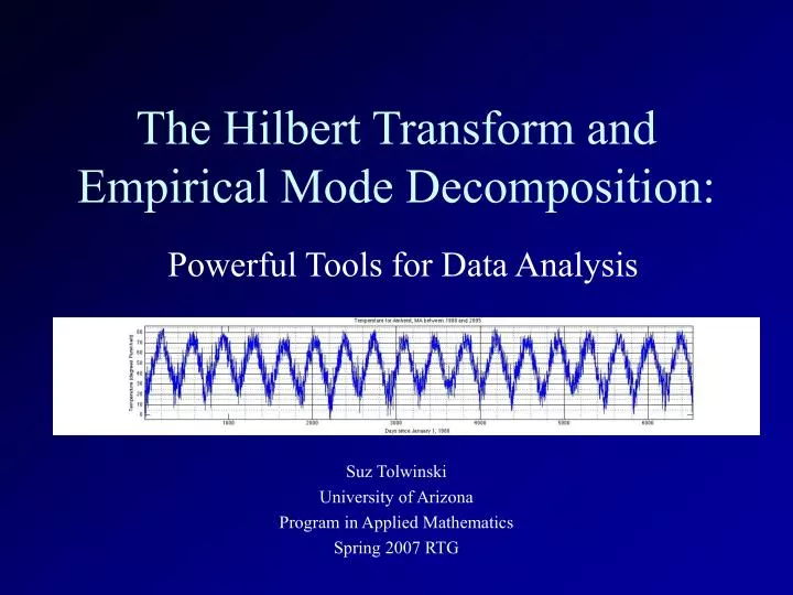
The Hilbert Transform and Empirical Mode Decomposition:. Powerful Tools for Data Analysis. Suz Tolwinski University of Arizona Program in Applied Mathematics Spring 2007 RTG. Deriving the Hilbert Transform.

E N D
The Hilbert Transform and Empirical Mode Decomposition: Powerful Tools for Data Analysis Suz Tolwinski University of Arizona Program in Applied Mathematics Spring 2007 RTG
Deriving the Hilbert Transform For f(z) = u(x,y) + iv(x,y) analytic on the upper half-plane, and decays at infinity: Cauchy’s Integral Formula + Decay of function + Clever rearrangement of terms : Relationship between u(x,y) and v(x,y) on R Define the Hilbert transform in similar spirit:
Another View of the Hilbert Transform. Looks like minus the convolution of f(t) with 1/πt. Apply Convolution Theorem for something more manageable in frequency space? Take away message: The Hilbert transform rotates a signal counter-clockwise by π/2 at every point in its positive frequency spectrum, and clockwise at all its negative frequencies.
Real Signals. A signal is any time-varying quantity containing information. Signals in nature are real. Real signals have even frequency spectra. This makes them difficult to analyze. We would like to know, how is the signal energy distributed in time and/or frequency space? For a signal with even frequency spectrum, -Mean frequency? -Spread of signal in frequency space? (Energy of s(t)= |s(t)|2 dt = |S()|2 d) Electrocardiographic signal in time and frequency domain
Analytic Signals. Have positive frequency spectrum only, so <>, spread in are meaningful quantities. We can construct an analytic signal corresponding to any real signal (takes only the positive frequencies): Frequency spectrum of a real signal. FANALYT.() = 1/2(F()+ sgn()F()) Then in the time domain, the analytic signal is given by Frequency spectrum of the corresponding analytic signal. fANALYT.(t) =1/2(f(t) + iH{f(t)}) Analytic signal can be represented as time-varying frequency and amplitude: fANALYT.(t) = A(t)ei(t) A(t) = (1/2f(t))2+1/2 (H{f(t)})2)1/2 (t) = tan-1(H{f(t)}/f(t))
Empirical Mode Decomposition of Real Signals. (Method due to N. Huang, 1998.) • Creates an adaptive decomposition of signal • Result is a generalized Fourier series • (Modes with time-varying amplitude and phase) • Components are called Intrinsic Mode Functions (IMFs) • IMFs satisfy two criteria by designs: • -Have only one zero between successive extrema • -Have zero “local mean” • EMD separates phenomena occurring on different time scales. • “Residue” shows overall trend in data.
Huang’s “Sifting Process”. Residue = s(t) I1(t) = Residue i = 1 k = 1 while Residue not equal zero or not monotone while Ii has non-negligible local mean U(t) = spline through local maxima of Ii L(t) = spline through local minima of Ii Av(t) = 1/2 (U(t) + L(t)) Ii(t) = Ii(t) - Av(t) i = i + 1 end IMFk(t) = Ii(t) Residue = Residue - IMFk k = k+1 end
Huang’s “Sifting Process”. Residue = s(t) I1(t) = Residue i = 1 k = 1 while Residue not equal zero or not monotone while Ii has non-negligible local mean U(t) = spline through local maxima of Ii L(t) = spline through local minima of Ii Av(t) = 1/2 (U(t) + L(t)) Ii(t) = Ii(t) - Av(t) i = i + 1 end IMFk(t) = Ii(t) Residue = Residue - IMFk k = k+1 end
Huang’s “Sifting Process”. Residue = s(t) I1(t) = Residue i = 1 k = 1 while Residue not equal zero or not monotone while Ii has non-negligible local mean U(t) = spline through local maxima of Ii L(t) = spline through local minima of Ii Av(t) = 1/2 (U(t) + L(t)) Ii(t) = Ii(t) - Av(t) i = i + 1 end IMFk(t) = Ii(t) Residue = Residue - IMFk k = k+1 end
Huang’s “Sifting Process”. Residue = s(t) I1(t) = Residue i = 1 k = 1 while Residue not equal zero or not monotone while Ii has non-negligible local mean U(t) = spline through local maxima of Ii L(t) = spline through local minima of Ii Av(t) = 1/2 (U(t) + L(t)) Ii(t) = Ii(t) - Av(t) i = i + 1 end IMFk(t) = Ii(t) Residue = Residue - IMFk k = k+1 end
Huang’s “Sifting Process”. Residue = s(t) I1(t) = Residue i = 1 k = 1 while Residue not equal zero or not monotone while Ii has non-negligible local mean U(t) = spline through local maxima of Ii L(t) = spline through local minima of Ii Av(t) = 1/2 (U(t) + L(t)) Ii(t) = Ii(t) - Av(t) i = i + 1 end IMFk(t) = Ii(t) Residue = Residue - IMFk k = k+1 end
Huang’s “Sifting Process”. Residue = s(t) I1(t) = Residue i = 1 k = 1 while Residue not equal zero or not monotone while Ii has non-negligible local mean U(t) = spline through local maxima of Ii L(t) = spline through local minima of Ii Av(t) = 1/2 (U(t) + L(t)) Ii(t) = Ii(t) - Av(t) i = i + 1 end IMFk(t) = Ii(t) Residue = Residue - IMFk k = k+1 end
Huang’s “Sifting Process”. Residue = s(t) I1(t) = Residue i = 1 k = 1 while Residue not equal zero or not monotone while Ii has non-negligible local mean U(t) = spline through local maxima of Ii L(t) = spline through local minima of Ii Av(t) = 1/2 (U(t) + L(t)) Ii(t) = Ii(t) - Av(t) (“residue”-->) i = i + 1 end IMFk(t) = Ii(t) Residue = Residue - IMFk k = k+1 end
Huang’s “Sifting Process”. Residue = s(t) I1(t) = Residue i = 1 k = 1 while Residue not equal zero or not monotone while Ii has non-negligible local mean U(t) = spline through local maxima of Ii L(t) = spline through local minima of Ii Av(t) = 1/2 (U(t) + L(t)) Ii(t) = Ii(t) - Av(t) i = i + 1 end IMFk(t) = Ii(t) Residue = Residue - IMFk k = k+1 end
Huang’s “Sifting Process”. Residue = s(t) I1(t) = Residue i = 1 k = 1 while Residue not equal zero or not monotone while Ii has non-negligible local mean U(t) = spline through local maxima of Ii L(t) = spline through local minima of Ii Av(t) = 1/2 (U(t) + L(t)) Ii(t) = Ii(t) - Av(t) i = i + 1 end IMFk(t) = Ii(t) Residue = Residue - IMFk k = k+1 end
Huang’s “Sifting Process”. Residue = s(t) I1(t) = Residue i = 1 k = 1 while Residue not equal zero or not monotone while Ii has non-negligible local mean U(t) = spline through local maxima of Ii L(t) = spline through local minima of Ii Av(t) = 1/2 (U(t) + L(t)) Ii(t) = Ii(t) - Av(t) i = i + 1 end IMFk(t) = Ii(t) Residue = Residue - IMFk k = k+1 end
Huang’s “Sifting Process”. Residue = s(t) I1(t) = Residue i = 1 k = 1 while Residue not equal zero or not monotone while Ii has non-negligible local mean U(t) = spline through local maxima of Ii L(t) = spline through local minima of Ii Av(t) = 1/2 (U(t) + L(t)) Ii(t) = Ii(t) - Av(t) i = i + 1 end IMFk(t) = Ii(t) Residue = Residue - IMFk k = k+1 end
Huang’s “Sifting Process”. Residue = s(t) I1(t) = Residue i = 1 k = 1 while Residue not equal zero or not monotone while Ii has non-negligible local mean U(t) = spline through local maxima of Ii L(t) = spline through local minima of Ii Av(t) = 1/2 (U(t) + L(t)) Ii(t) = Ii(t) - Av(t) i = i + 1 end IMFk(t) = Ii(t) Residue = Residue - IMFk k = k+1 end
Huang’s “Sifting Process”. Residue = s(t) I1(t) = Residue i = 1 k = 1 while Residue not equal zero or not monotone while Ii has non-negligible local mean U(t) = spline through local maxima of Ii L(t) = spline through local minima of Ii Av(t) = 1/2 (U(t) + L(t)) Ii(t) = Ii(t) - Av(t) i = i + 1 end IMFk(t) = Ii(t) Residue = Residue - IMFk k = k+1 end
Huang’s “Sifting Process”. Residue = s(t) I1(t) = Residue i = 1 k = 1 while Residue not equal zero or not monotone while Ii has non-negligible local mean U(t) = spline through local maxima of Ii L(t) = spline through local minima of Ii Av(t) = 1/2 (U(t) + L(t)) Ii(t) = Ii(t) - Av(t) i = i + 1 end IMFk(t) = Ii(t) Residue = Residue - IMFk k = k+1 end
The Hilbert Spectrum Now that we have a set of IMFs; construct their analytic counterparts using the Hilbert transform. Now we can look at f(t) in time and frequency space simultaneously. Instantaneous frequency is given by the derivative of the phase angle. The Hilbert spectrum H(,t) gives the instantaneous amplitude (~energy) as a function of frequency. A plot of H(,t) provides an intuitive, visual representation of the signal in time and frequency.
Real-World Example: Temperature Data from Amherst, MA from 1988 - 2005.
Physical Interpretation of IMFs for Amherst Temperature Data. IMF 8 IMF 5
Huang-Hilbert Spectrum for EMD of Amherst Temperature Data -Most of the signal information contained in the bottom 10% of all frequencies represented -Can we make a correspondence between what we see here and the IMFs of the decomposition? -This would help identify which modes are important in determining the character of the data.
Increasing Frequencies: Decreasing Information! IMF 4 IMF 5 IMF 6
Bibliography. • Langton, C. Hilbert Transform, Anayltic Signal and the Complex Envelope Signal Processing and Simulation Newsletter, 1999. http://www.complextoreal.com/tcomplex.htm • Electrocardiograph signal graphic: http://www.neurotraces.com/scilab/scilab2/node61.html • MATLAB code used for all computations, and “sifting” graphics: • Rilling, G. MATLAB code for computation of EMD and illustrative slides. • http://perso.ens lyon.fr/patrick.flandrin/emd.html • Temperature data from Amherst, MA: • Williams, C.N., Jr., M.J. Menne, R.S. Vose, and D.R. Easterling. 2006. United States • Historical Climatology Network Daily Temperature, Precipitation, and Snow Data. • ORNL/CDIAC-118, NDP-070. Online at [http://cdiac.ornl.gov/epubs/ndp/ushcn/usa.html]; site MA190120 • “Burning Globe” graphic: http://river2sea72.wordpress.com/2007/03/24/its-not-all-about-carbon-or-is-it/