Download
1 / 30
310 likes | 507 Vues
Surface reflectance over Land. Eric Vermote NASA GSFC Code 619 Eric.f.vermote@nasa.gov . . A Land Climate Data Record Multi instrument/Multi sensor Science Quality Data Records used to quantify trends and changes. 81. 82. 83. 84. 85. 86. 87. 88. 89. 90. 91. 92. 93. 94. 95.

E N D
Surface reflectance over Land Eric Vermote NASA GSFC Code 619 Eric.f.vermote@nasa.gov . MODIS Science Team Meeting , April 29 – May 1 , 2014 , Columbia, MD
A Land Climate Data Record Multi instrument/Multi sensor Science Quality Data Records used to quantify trends and changes 81 82 83 84 85 86 87 88 89 90 91 92 93 94 95 96 97 98 99 00 01 02 03 04 05 06 07 08 09 10 11 12 13 14 15 16 17 N16 N17 METOP AVHRR N07 N09 N11 N09 N14 N16 SPOT VEGETATION Terra MODIS Aqua AVHRR (GAC) 1982-1999 + 2003-2006 MODIS (MO(Y)D09 CMG) 2000-present VIIRS 2011 – 2025 SPOT VEGETATION 1999-2000 Sentinel 3 2014 NPP VIIRS JPSS 1 Sentinel 3 • Emphasis on data consistency – characterization rather than degrading/smoothing the data MODIS Science Team Meeting , April 29 – May 1 , 2014 , Columbia, MD
Land Climate Data Record (Approach) Needs to address geolocation,calibration, atmospheric/BRDF correction issues ATMOSPHERIC CORRECTION CALIBRATION BRDF CORRECTION Degradation in channel 1 (from Ocean observations) Channel1/Channel2 ratio (from Clouds observations) Pinatubo El Chichon MODIS Science Team Meeting , April 29 – May 1 , 2014 , Columbia, MD
Goals/requirements for atmospheric correction • Ensuring compatibility of missions in support of their combined use for science and application (example Climate Data Record) • A prerequisite is the careful absolute calibration that could be insured by cross-comparison over specific sites (e.g. desert) • We need consistency between the different AC approaches and traceability but it does not mean the same approach is required – (i.e. in most cases it is not practical) • Have a consistent methodology to evaluate surface reflectance products: • AERONET sites • Ground measurements • In order to meaningfully compare different reflectance product we need to: • Understand their spatial characteristics • Account for directional effects • Understand the spectral differences • One can never over-emphasize the need for efficient cloud/cloud shadow screening MODIS Science Team Meeting , April 29 – May 1 , 2014 , Columbia, MD
Surface Reflectance (MOD09) The Collection 5 atmospheric correction algorithm is used to produce MOD09 (the surface spectral reflectance for seven MODIS bands as it would have been measured at ground level if there were no atmospheric scattering and absorption). • The Collection 5 AC algorithm relies on • the use of very accurate (better than 1%) vector radiativetransfer modeling of the coupled atmosphere-surfacesystem • the inversion of key atmospheric parameters (aerosol, water vapor) Home page: http://modis-sr.ltdri.org MODIS Science Team Meeting , April 29 – May 1 , 2014 , Columbia, MD
6SV Validation Effort • The complete 6SV validation effort is summarized in three manuscripts: • Kotchenova, S. Y., Vermote, E. F., Matarrese, R., & KlemmJr, F. J. (2006). Validation of a vector version of the 6S radiative transfer code for atmospheric correction of satellite data. Part I: Path radiance. Applied Optics, 45(26), 6762-6774. • Kotchenova, S. Y., & Vermote, E. F. (2007). Validation of a vector version of the 6S radiative transfer code for atmospheric correction of satellite data. Part II. Homogeneous Lambertian and anisotropic surfaces. Applied Optics, 46(20), 4455-4464. • Kotchenova, S. Y., Vermote, E. F., Levy, R., & Lyapustin, A. (2008). Radiative transfer codes for atmospheric correction and aerosol retrieval: intercomparison study. Applied Optics, 47(13), 2215-2226. MODIS Science Team Meeting , April 29 – May 1 , 2014 , Columbia, MD
Vector 6S Monte Carlo (benchmark) Dave Vector SHARM (scalar) RT3 Coulson’s tabulated values (benchmark) Code Comparison Project All information on this project can be found athttp://rtcodes.ltdri.org MODIS Science Team Meeting , April 29 – May 1 , 2014 , Columbia, MD
Error Budget Goal: to estimate the accuracy of the atmospheric correction under several scenarios Reference:Vermote, E. F. & El Saleous, N. Z. (2006). Operational atmospheric correction of MODIS visible to middle infrared land surface data in the case of an infinite Lambertian target, In: Earth Science Satellite Remote Sensing, Science and Instruments, (eds: Qu. J. et al), vol. 1, chapter 8, 123 - 153. MODIS Science Team Meeting , April 29 – May 1 , 2014 , Columbia, MD
Error budget Example: Calibration Uncertainties We simulated an error of ±2% in the absolute calibration across all 7 MODIS bands. Results: The overall error stays under 2% in relative for all aerosol cases considered. (In all study cases, the results are presented in the form of tables and graphs.) Table (example): Error on the surface reflectance (x 10,000) due to uncertainties in the absolute calibration for the Savanna site. MODIS Science Team Meeting , April 29 – May 1 , 2014 , Columbia, MD
Overall Theoretical Accuracy Overall theoretical accuracy of the atmospheric correction method considering the error source on calibration, ancillary data, and aerosol inversion for 3 τaer = {0.05 (clear), 0.3 (avg.), 0.5 (hazy)}: The selected sites are Savanna (Skukuza), Forest (Belterra), and Semi-arid (Sevilleta). The uncertainties are considered independent and summed in quadratic. MODIS Science Team Meeting , April 29 – May 1 , 2014 , Columbia, MD
Methodology for evaluating the performance of MOD09 To first evaluate the performance of the MODIS Collection 5 SR algorithms, we analyzed 1 year of Terra data (2003) over 127 AERONET sites (4988 cases in total). Methodology: Subsets of Level 1B data processed using the standard surface reflectance algorithm comparison Reference data set Atmospherically corrected TOA reflectances derived from Level 1B subsets If the difference is within ±(0.005+0.05ρ), the observation is “good”. AERONET measurements (τaer, H2O, particle distribution Refractive indices,sphericityeri) Vector 6S http://mod09val.ltdri.org/cgi-bin/mod09_c005_public_allsites_onecollection.cgi MODIS Science Team Meeting , April 29 – May 1 , 2014 , Columbia, MD
Validation of MOD09 Comparison between the MODIS band 1 surface reflectance and the reference data set. The circle color indicates the % of comparisons within the theoretical MODIS 1-sigma error bar: green > 80%, 65% < yellow <80%, 55% < magenta < 65%, red <55%. The circle radius is proportional to the number of observations. MODIS Science Team Meeting , April 29 – May 1 , 2014 , Columbia, MD
Toward a quantitative assessment of performances (APU) 1,3 Millions 1 km pixels were analyzed for each band. Red = Accuracy (mean bias) Green = Precision (repeatability) Blue = Uncertainty (quadatric sum of A and P) On average well below magenta theoretical error bar MODIS Science Team Meeting , April 29 – May 1 , 2014 , Columbia, MD
Improving the aerosol retrieval (by using a ratio map instead of fixed ratio) in collection 6 well reflected in APU metrics ratio band3/band1 derived using MODIS top of the atmosphere corrected with MISR aerosol optical depth MODIS Science Team Meeting , April 29 – May 1 , 2014 , Columbia, MD
Improving the aerosol retrieval in collection 6 reflected in APU metrics MODIS Science Team Meeting , April 29 – May 1 , 2014 , Columbia, MD
MODIS product and validation methodology used to evaluate other surface reflectance product: example LANDSAT TM/ETM+ • WELD (D. Roy) 120 acquisitions over 23 AERONET sites (CONUS) JunchangJu, David P. Roy, Eric Vermote, Jeffrey Masek, ValeriyKovalskyy, Continental-scale validation of MODIS-based and LEDAPS Landsat ETM+ atmospheric correction methods, Remote Sensing of Environment (2012), Available online 10 February 2012, ISSN 0034-4257, 10.1016/j.rse.2011.12.025. • GFCC: Comparison with MODIS SR products • GLS 2000 demonstration Min Feng, Chengquan Huang, SaurabhChannan, Eric F. Vermote, Jeffrey G. Masek, John R. Townshend, Quality assessment of Landsat surface reflectance products using MODIS data, Computers & Geosciences, Volume 38, Issue 1, January 2012, Pages 9-22, ISSN 0098-3004, 10.1016. • GLS 2005 (TM and ETM+) Min Feng Joseph O. Sexton, Chengquan Huang, Jeffrey G. Masek, Eric F. Vermote, FengGao, RaghuramNarasimhan, SaurabhChannan, Robert E. Wolfe, John R. Townshend ,Global, long-term surface reflectance records from Landsat: a comparison of the Global Land Survey and MODIS surface reflectance datasets. Remote Sensing of the Environment (in review) MODIS Science Team Meeting , April 29 – May 1 , 2014 , Columbia, MD
WELD/LEDAPS/LDCM results (Red-band3) LEDAPS WELD uses MODIS aerosol LDCM MODIS Science Team Meeting , April 29 – May 1 , 2014 , Columbia, MD
Continuous analysis of time series allow an independent assessment of precision Evaluation over AERONET (2003) 0.007 <Precision < 0.017 Independent evaluation of the precision Over 2000-2004 CMG daily time series FOREST Precision=0.016 CROPS SAVANNA Precision=0.013 Precision=0.01 MODIS Science Team Meeting , April 29 – May 1 , 2014 , Columbia, MD
Quantification of time series noise • One can then compute a “noise” from the quadratic sum of the difference between the measurement and their interpolated counterpart: • We use this definition in the following to quantify the time series quality For each triplet of observations, one can estimate middle one from the earlier and later: MODIS Science Team Meeting , April 29 – May 1 , 2014 , Columbia, MD
Evaluation of VJB BRDF correction at CMG spatial resolution (0.05 deg) over AERONET sites (Bréon and Vermote,2012) Examples over 3 sites Black: Original Red: VJB Blue: MCD43A2 Green: average Results over 115 sites MODIS Science Team Meeting , April 29 – May 1 , 2014 , Columbia, MD
Evaluation of BRDF correction at native spatial resolution (500m) over Australia MODIS data are distributed as “tiles” (10° of lat.) To limit data volume, we focus on a single tile Select a tile over Eastern Australia for (i) variety of surface cover, (ii) number of clear observations, (iii) low aerosol load MODIS Science Team Meeting , April 29 – May 1 , 2014 , Columbia, MD
Impact of spatial scale The noise of the corrected time series is much larger than that we obtained earlier using CMG (Climate Modeling Grid : 5 km) lower resolution data. We show here a comparison of the noise obtained at the full resolution against that obtained when aggregating 5x5 pixels. MODIS Science Team Meeting , April 29 – May 1 , 2014 , Columbia, MD
Noise vs Spatial heterogeneity There is a very strong correlation between the spatial heterogeneity (quantified here as the 3x3 standard deviation) and the noise on the corrected time series. Clearly, the spatial heterogeneity affects the quality of the time series and there is an easy explanation for that (gridding and FOV) MODIS Science Team Meeting , April 29 – May 1 , 2014 , Columbia, MD
Impact of spatial scale The “noise” of the time series decreases when the spatial aggregation increases. There seems to be an optimal scale at 2 km (4x4 pixels) MODIS Science Team Meeting , April 29 – May 1 , 2014 , Columbia, MD
Use of BRDF correction for product cross-comparison MODIS Science Team Meeting , April 29 – May 1 , 2014 , Columbia, MD
Continuous monitoring and assessment of instrument performance is also important CALIBRATION MODIS Science Team Meeting , April 29 – May 1 , 2014 , Columbia, MD
Continuous monitoring and assessment of instrument performance is also important POLARIZATION EFFECT (BAND8) MODIS Science Team Meeting , April 29 – May 1 , 2014 , Columbia, MD
Continuous monitoring and assessment of instrument performance is also important POLARIZATION EFFECT (Aerosol optical thickness) MODIS Science Team Meeting , April 29 – May 1 , 2014 , Columbia, MD
Monitoring of product quality (exclusion conditions cloud mask using CALIOP) MODIS Science Team Meeting , April 29 – May 1 , 2014 , Columbia, MD
Conclusions Surface reflectance (SR) algorithm is mature and pathway toward validation and automated QA is clearly identified. Algorithm is generic and tied to documented validated radiative transfer code so the accuracy is traceable enabling error budget. The use of BRDF correction enables easy cross-comparison of different sensors (MODIS,VIIRS,AVHRR, LDCM, Landsat, Sentinel 2 ,Sentinel 3…) Cloud and cloud shadow mask validation protocol needs to be fully developed. MODIS Science Team Meeting , April 29 – May 1 , 2014 , Columbia, MD