Download
1 / 55
560 likes | 804 Vues
Multiple Input Production Economics for Farm Management. AAE 320 Paul D. Mitchell. Multiple Input Production. Most agricultural production processes have more than one input, e.g., capital, labor, land, or N, P, K fertilizer, plus herbicides, insecticides, tillage, water, etc.

E N D
Multiple Input Production Economics for Farm Management AAE 320 Paul D. Mitchell
Multiple Input Production • Most agricultural production processes have more than one input, e.g., capital, labor, land, or N, P, K fertilizer, plus herbicides, insecticides, tillage, water, etc. • How do you decide how much of each input to use when you are choosing more than one input? • We will derive the Equal Margin Principle and show its use to answer this question
Equal Margin Principle • Will derive using calculus so you see where it comes from • Applies whether you use a function or not, so can apply Equal Margin Principle to the tabular form of the multiple input production schedule • Multivariate calculus requires use of Partial Derivatives, so let’s review
Partial Derivatives • Derivative of function that has more than one variable • What’s the derivative of f(x,y)? Depends on which variable you are talking about. • Remember a derivative is the slope • Derivative of f(x,y) with respect to x is the slope of the function in the x direction • Derivative of f(x,y) with respect to y is the slope of the function in the y direction
Partial Derivatives • Think of a hill; its elevation Q is a function of the location in latitude (x) and in longitude (y): Q = f(x,y) • At any spot on the hill, defined by a latitude-longitude pair (x,y), the hill will have a slope in the x direction and in the y direction • Slope in x direction: dQ/dx = fx(x,y) • Slope in y direction: dQ/dy = fy(x,y)
Q Q=f(X,Y) Y X Source: “Neoclassical Theories of Production” on The History of Economic Thought Website: http://cepa.newschool.edu/het/essays/product/prodcont.htm
Partial Derivatives • Notation: if have Q = f(x,y) • First Partial Derivatives • dq/dx = fx(x,y) and dQ/dy = fy(x,y) • Second (Own) Partial Derivative • d2Q/dx2 = fxx(x,y) and d2Q/dy2 = fyy(x,y) • Second Cross Partial Derivative • d2Q/dxdy = fxy(x,y)
Partial Derivatives • Partial derivatives are the same as regular derivatives, just treat the other variables as constants • Q = f(x,y) = 2 + 3x + 6y – 2x2 – 3y2 – 5xy • When you take the derivative with respect to x, treat y as a constant and vice versa • fx(x,y) = 3 – 4x – 5y • fy(x,y) = 6 – 6y – 5x
Think Break #5 • Give the 1st and 2nd derivatives [fx(x,y), fy(x,y),, fxx(x,y), fyy(x,y), fxy(x,y)] of each: • f(x,y) = 7 + 5x + 2y – 5x2 – 4y2 – 11xy • f(x,y) = – 5 – 2x + y – x2 – 3y2 + 2xy
Equal Margin Principle • Given production function Q = f(x,y), find (x,y) to maximize p = pf(x,y) – rxx – ryy – K • FOC’s: dp/dx = 0 and dp/dy = 0 and solve for pair (x,y) • dp/dx = pfx(x,y) – rx = 0 • dp/dy = pfy(x,y) – ry = 0 • Just p x MPx = rx and p x MPy = ry • Just MPx = rx/p and MPy = ry/p • These still hold, but we also have more
Equal Margin Principle • Profit Maximization again implies • p x MPx = rx and p x MPy = ry • Note that p x MPx = rx depends on y and p x MPy = ry depends on x • Note that two equations and both must be satisfied, so rearrange by making the ratio
Equal Margin Principle • Equal Margin Principle is expressed mathematically in two ways 1) MPx/rx = MPy/ry 2) MPx/MPy = rx/ry • Ratio of MPi/ri must be equal for all inputs • Ratio of MP’s must equal input price ratio
Intuition: Corn Example • MPi is bu of corn per lb of N fertilizer (bu/lb) • ri is $ per lb of N fertilizer ($/lb) • MPi/ri is bu of corn per $ spent on N fertilizer (bu/lb)/ ($/lb) = bu/$ • MPi/riis how many bushels of corn you get for the last dollar spent on N fertilizer • MPx/rx = MPy/ry means use inputs so that the last dollar spent on each input gives the same extra output
Intuition: Corn Example • MPx is bu of corn from last lb of N fert. (bu/lb N) • MPy is bu of corn from last lb of P fert. (bu/lb P) • MPx/MPy = (lbs P/lbs N) is how much P need if cut N by 1 lb and want to keep output constant • Ratio of marginal products is the substitution rate between N and P in the production process
Intuition: Corn Example • rx is $ per lb of N fertilizer ($/lb N) • ry is $ per lb of P fertilizer ($/lb P) • rx/ry is ($/lb N)/($/lb P) = lbs P/lbs N, or the substitution rate between N and P in the market • MPx/MPy = rx/ry means use inputs so that the substitution rate between inputs in the production process is the same as the substitution rate between inputs in the market
Marginal Rate of Technical Substitution • The ratio of marginal products (MPx/MPy) is the substitution rate between inputs in the production process • MPx/MPy is called the Marginal Rate of Technical Substitution (MRTS): the input substitution rate at the margin for the production technology • If cut X by one unit, how much must you increase Y to keep output the same • Optimality condition MPx/MPy = rx/ry means set substitution rates equal
Equal Margin Principle Intuition • MPx/rx = MPy/ry means use inputs so the last dollar spent on each input gives the same extra output at the margin • Compare to p x MP = r or VMP = r • MPx/MPy = rx/ry means use inputs so the substitution rate at the margin between inputs is the same in the production process as in the market place • Compare to MP = r/p
Equal Margin PrincipleGraphical Analysis via Isoquants • Isoquant (“equal-quantity”) plot or function representing all combinations of two inputs producing the same output quantity • Intuition: Isoquants are the two dimensional “contour lines” of the three dimensional production “hill” • First look at in Theory, then a Table
Isoquants in Theory Input Y ~ Output Q = Q Input X
Isoquants and MPx/MPy Isoquant Slope = DY/DX = Substitutionrate between X and Y at the margin. If reduce X by the amount DX, then must increase Y by the amount DY to keep output fixed DY Input Y DX ~ Output Q = Q Input X
Isoquants and MPx/MPy Isoquant slope = dY/dX dY/dX = –(dQ/dX)/(dQ/dY) dY/dX = – MPx/MPy = – Ratio of MP’s Isoquant Slope = – MRTS DY Need minus sign since marginal products are positive and slope is negative Input Y DX ~ Output Q = Q Input X
Isoquants and MPx/MPy = rx/ry • Isoquant slope (– MPx/MPy) is (minus) the substitution rate between X and Y at the margin • Thus define minus the isoquant slope as the “Marginal Rate of Technical Substitution” (MRTS) • Price ratio rx/ry is the substitution rate between X and Y (at the margin) in the market place • Economically optimal use of inputs sets these substitution rates equal, or MPx/MPy = rx/ry
Isoquants and MPx/MPy = rx/ry • Find the point of tangency between the isoquant and the input price ratio • Kind of like the MP = r/p: tangency between the production function and input-output price ratio line Input Y ~ Output Q = Q Slope = – MPx/MPy = – rx/ry Input X
Soybean meal and corn needed for 125 lb feeder pigs to gain 125 lbs Which feed ration do you use?
MRTS = As increase Soybean Meal, how much can you decrease Corn and keep output constant? • Can’t use MRTS = – MPx/MPysince DQ = 0 on an isoquant • Use MRTS = – DY/DX • DX = (SoyM2 – SoyM1) • DY = (Corn2 – Corn1) = – (294.6 – 300.6)/(45 – 40) = –(284.4 – 289.2)/(55 – 50) Interpretation: If increase soybean meal 1 lb, decrease corn by 1.20 or 0.96 lbs and keep same gain on hogs
Economically Optimal input use is where MRTS = input price ratio, or – DY/DX = rx/ry (Same as MPx/MPy = rx/ry) Soybean Meal Price $176/ton = $0.088/lb Corn Price $2.24/bu = $0.04/lb Ratio: 0.088/0.04 = 2.20 lbs corn/lbs soy Keep straight which is X and which is Y!!!
Intuition • What does – DY/DX = rx/ry mean? • Ratio – DY/DX is how much less Y you need if you increase X, or the MRTS • Cross multiply to get – DYry = DXrx • – DYry = cost savings from decreasing Y • DXrx = cost increase from increasing X • Keep sliding down the isoquant (decreasing Y and increasing X) as long as the cost saving exceeds the cost increase
Main Point on MRTS • When you have information on inputs needed to generate the same output, you can identify the optimal input combination • Theory: (MRTS) MPx/MPy = rx/ry • Practice: (isoquant slope) – DY/DX = rx/ry • Note how the input in the numerator and denominator changes between theory and practice
Think Break #6 The table is rations of grain and hay that put 300 lbs of gain on 900 lb steers. 1) Fill in the missing MRTS 2) If grain is $0.04/lb and hay is $0.03/lb, what is the economically optimal feed ration?
Summary • Can identify economically optimal input combination using tabular data and prices • Requires input data on the isoquant, i.e., different feed rations that generate the same amount of gain • Again: use calculus to fill in gaps in the tabular form of isoquants
Types of Substitution • Perfect substitutes: soybean meal & canola meal, corn & sorghum, wheat and barley • Imperfect substitutes: corn & soybean meal • Non-substitutes/perfect complements: tractors and drivers, wire and fence posts
Perfect Substitutes • MRTS (slope of isoquant) is constant • Examples: canola meal and soybean meal, or corn and sorghum in a feed ration • Constant conversion between two inputs • 2 pounds of canola meal = 1 pound of soybean meal: – DCnla/DSoyb = 2 • 1.2 bushels of sorghum = 1 bu corn – DSrgm/DCorn = 1.2
Economics of Perfect Substitutes • MRTS = rx/ry still applies MRTS = k: – DY/DX = – DCnla/DSoyb = 2 • If rx/ry < k, use only input x • soybean meal < twice canola meal price • soyb meal $200/cwt, cnla meal $150/cwt • If rx/ry > k, use only input y • soybean meal > twice canola meal price • soyb meal $200/cwt, cnla meal $90/cwt • If rx/ry = k, use any x-y combination
Use only Canola Meal rx/ry > 2 Perfect Substitutes: Graphics Use any combination of Canola or Soybean Meal 2 1 rx/ry = 2 Canola Meal Use only Soybean Meal rx/ry < 2 Soybean Meal
Economics of Imperfect Substitutes This the case we already did! Input Y Input X
Perfect Complements, or Non-Substitutes • No substitution is possible • The two inputs must be used together • Without the other input, neither input is productive, they must be used together • Tractors and drivers, fence posts and wire, chemical reactions, digger and shovel • Inputs used in fixed proportions 1 driver for 1 tractor
Economics of Perfect Complements • MRTS is undefined, the price ratio rx/ry does not identify the optimal combination • Leontief Production Function Q = min(aX,bY): • Marginal products of inputs = 0 • Either an output quota or a cost budget, with the fixed input proportions, define how much of the inputs to use
Perfect Complements: Graphics Price ratio does not matter rx/ry > 2 Drivers rx/ry < 2 Tractors
Multiple Input Production with Calculus • Use calculus with production function to find the optimal input combination • General problem we’ve seen: Find (x,y) to maximize p = pf(x,y) – rxx – ryy – K • Will get FOC’s, one for each choice variable, and SOC’s are more complicated • Assume price p = 10, price of x (rx) = 2 and price of y (ry) = 3
Multiple Input Production with Calculus • Max 10(7 + 9x + 8y – 2x2 – y2 – 2xy) – 2x – 3y – 8 • FOC1: 10(9 – 4x – 2y) – 2 = 0 • FOC2: 10(8 – 2y – 2x) – 3 = 0 • Find the (x,y) pair that satisfies these two equations • Same as finding where the two lines from the FOC’s intersect
FOC1: 10(9 – 4x – 2y) – 2 = 0 • FOC2: 10(8 – 2y – 2x) – 3 = 0 1) Solve FOC1 for x 88 – 40x – 20y = 0 40x = 88 – 20y x = (88 – 20y)/40 = 2.2 – 0. 5y 2) Substitute this x into FOC2 and solve for y 77 – 20y – 20x = 0 77 – 20y – 20(2.2 – 0.5y) = 0 77 – 20y – 44 + 10y = 0 33 – 10y = 0, or 10y = 33, or y = 3.3 3) Calculate x: x = 2.2 – 0. 5y = 2.2 – 0.5(3.3) = 0.55
Second Order Conditions • SOC’s are more complicated with multiple inputs, must look at curvature in each direction, plus the “cross” direction (to ensure do not have a saddle point). 1) Own second derivatives must be negative for a maximum: fxx < 0, fyy < 0 (both > 0 for a minimum) 2) Another condition: fxxfyy – (fxy)2 > 0
FOC1: 10(9 – 4x – 2y) – 2 = 0 • FOC2: 10(8 – 2y – 2x) – 3 = 0 • Second Derivatives 1) fxx: 10(– 4) = – 40 2) fyy: 10(– 2) = – 20 3) fxy: 10(– 2) = – 20 SOC’s 1) fxx = – 40 < 0 and fyy = – 20 < 0 2) fxxfyy – (fxy)2 > 0 (– 40)(– 20) – (– 20)2 = 800 – 400 > 0 Solution x = 0.55 and y = 3.3 is a maximum
Milk Production • M = – 25.9 + 2.56G + 1.05H – 0.00505G2 – 0.00109H2 – 0.00352GH • M = milk production (lbs/week) • G = grain (lbs/week) • H = hay (lbs/week) • Milk $14/cwt, Grain $3/cwt, Hay $1.50/cwt • What are the profit maximizing inputs? (Source: Heady and Bhide 1983)
Milk Profit Function • p = 0.14(– 25.9 + 2.56G + 1.05H – 0.00505G2 – 0.00109H2 – 0.00352GH) – 0.03G – 0.015H • FOC’s 0.14(2.56 – 0.0101G – 0.00352H) – 0.03 = 0 0.14(1.05 – 0.00218H – 0.00352G) – 0.015 = 0 • Alternative: jump to optimality conditions MPG = rG/p and MPH = rH/p MPG = 2.56 – 0.0101G – 0.00352H = rG/p = 0.214 MPH = 1.05 – 0.00218H – 0.00352G = rH/p = 0.107
Solve FOC1 for H: 2.56 – 0.0101G – 0.00352H = 0.214 2.346 – 0.0101G = 0.00352H H = (2.346 – 0.0101G)/0.00352 H = 666 – 2.87G Substitute this H into FOC2 and solve for G: 1.05 – 0.00218H – 0.00352G = 0.107 0.943 – 0.00218(666 – 2.87G) – 0.00352G = 0 0.943 – 1.45 + 0.00626G – 0.00352G = 0 0.00274G – 0.507 = 0 G = 0.507/0.00274 = 185 lbs/week
Substitute this G into the equation for H H = 666 – 2.87G H = 666 – 2.87(185) H = 666 – 531 = 135 lbs/week Check SOC’s pGG = – (0.14)0.0101 = – 0.001414 < 0 pHH = – (0.14)0.00218 = – 0.000305 < 0 pGH = – (0.14)0.00352 = – 0.000493 pGGpHH – (pGH)2 = 1.88 x 10⁻⁷ > 0 SOC’s satisfied for a maximum