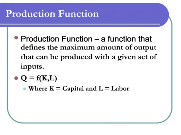
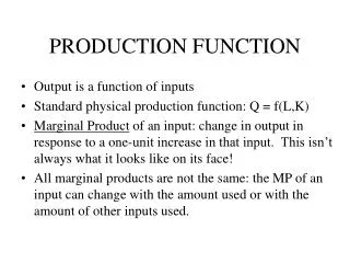
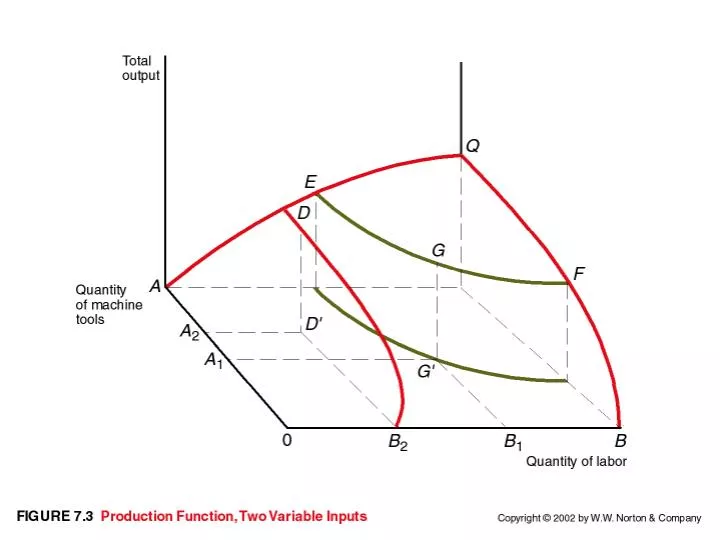
Production Function Multiple Variable Input

2. Production Function Multiple Variable Input • The 3D production function can be compressed into a set of isoquants plotted in a 2D (K,L) space. • An isoquant shows all the input mixes of (L,K) that produce the same amount of Q. • One isoquant for each level of Q • Isoquants have negative slope: more output from one input can offset less output from the other input

4. Isoquant • The shape of the isoquant reveals the degree of substitution between the inputs. • If the technology allows for perfect substitution between labor and capital, the isoquants are straight lines. • The inputs can substitute each other at the same rate to produce the same output. e.g. each unit of K can always be replaced by 2 units of L.

5. Isoquant • In reality, inputs are imperfect substitutes and the isoquants are convex to the origin. • Check: as you move up an isoquant in Fig 7.4, you need to use more and more capital to replace each unit of labor in order to stay on the same isoquant. • The magnitude of the slope of the isoquant is greater as you move “up” an isoquant.

7. Isoquant • Slope of an isoquantdK/dL is called the marginal rate of technical substitution. • MRTS is the amount of capital input (dK) needed to replace an amount of labor input (dL) to keep the same level of output: it measures the degree of substitution. • Q = Q(K, L). • As you move “up” along an isoquant, the total differential of Q is zero

8. Isoquant • dQ = (∂Q/∂L) (dL) + (∂Q/∂K) (dK) = 0 (MPL) (dL) + (MPK) (dK) = 0 (dK)/dL = - MPL/MPK < 0 • MRTS at different points on the isoquant is different since MPL and MPK are changing. • As you move “up” an isoquant, MRTS becomes larger “in magnitude” (more negative).

9. Isoquant • This is the result of the law of diminishing marginal productivity (LDMP). • LDMP states that “as you increase the amount of one input while keeping other inputs fixed, the marginal product of this input declines with output. • LDMP is a physical constraint – we can’t escape from it.

10. Isoquant • If LDMP is true, so is a weaker version of it: “as you increase the amount of one input while reducing other inputs, the marginal product of this input declines with output. • As we use less labor and more capital inputs along an isoquant, MPK, MPL  • MRTS = (dK)/dL = - MPL/MPK • “magnitude” of MRTS (more negative)

11. Optimal level of Input Mix to EmployMultiple variable input • For a profit max output Q, there are now many input mixes of L and K (along the isoquant for this output Q) that can be used to produce Q • Which input mix is cheapest? You need to take into account inputs prices

12. Isocost line • The amount of input you can employed depends on (1) their prices and (2) budget. • Define: an isocost line consists of all the input mixes (L, K) that can be employed with an expenditure budget M and a set of inputs prices of PL and PK.

13. Isocost line • Isocost line are all the (L, K) such that • PLL + PKK = M • K= M/PK – (PL/PK)L • Plot this eqt in the K-L space • Slope of isocost line = – (PL/PK) • X-axis intercept = M/PL • Y-axis intercept = M/PK

15. Isocost line • If M double, the line shifts out parallelly and the intercepts doubled (same effect if inputs prices are halved) • If both M and input prices are doubled, the isocost line is unchanged • If the price of labor inputs , the isocost line rotate: steeper and the x-axis intercept decreases.

16. Optimal level of Input (Mix) to EmployMultiple variable input • Suppose we know the profit max output Q. • Plot the isoquant of Q • Given input prices PL and PK, plot several isocost lines, each corresponds to a different expenditure budget M • The optimal input mix is one such that the isocost line just “touch” the isoquant of Q