Download
1 / 51
520 likes | 699 Vues
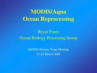
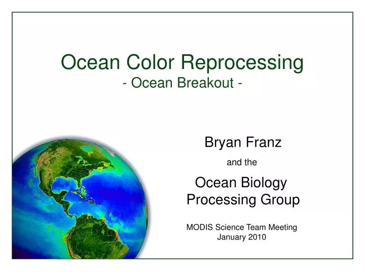
Ocean Color Reprocessing - Ocean Breakout -. Bryan Franz and the Ocean Biology Processing Group. MODIS Science Team Meeting January 2010. Ocean Color Reprocessing. Highlights: sensor calibration updates regeneration of all sensor bandpass quantities new aerosol models based on AERONET

E N D
Ocean Color Reprocessing - Ocean Breakout - Bryan Franz and the Ocean Biology Processing Group MODIS Science Team Meeting January 2010
Ocean Color Reprocessing Highlights: • sensor calibration updates • regeneration of all sensor bandpass quantities • new aerosol models based on AERONET • improved turbid-water atmospheric correction algorithm • accounting for atmospheric NO2 absorption • updated chlorophyll a and Kd algorithms based on NOMAD v2 • expanded product suite • maximizing consistency in all processing phases Scope: SeaWiFS, MODISA, MODIST, OCTS, CZCS • Status: • SeaWiFS reprocessing completed November 2009 • MODISA to begin next week, completed in February-March
Expanded MODIS Product Suite NEW OLD Rrs(412) Rrs(443) Rrs(469) Rrs(488) Rrs(531) Rrs(547) Rrs(555) Rrs(645) Rrs(667) Rrs(678) land bands revised band center • nLw(l) • Chlorophyll a • Kd(490) • Ångstrom • AOT • Epsilon • Rrs(l) • Chlorophyll a • Kd(490) • Ångstrom • AOT • POC • PIC • CDOM_index • PAR • iPAR • Fluorescence LH • Fluorescence QY
New Aerosol Models • based on AERONET size distributions & albedos • vector RT code accounting for polarization (Ahmad-Fraser) • 80 models (8 humidities x 10 size fractions) • model selection now descriminated by relative humidity • revised vicarious calibration assumption (a=0.65 at Tahiti) Old S&F Size Distributions New AERONET-based Size Distributions c50 c90 Ahmad, Z., B. A. Franz, C. R. McClain, E. J. Kwiatkowska, J. Werdell, E. Shettle, and B. N. Holben (2010). New aerosol models for the retrieval of aerosol optical thickness and normalized water-leaving radiances from the SeaWiFS and MODIS sensors over coastal regions and Open Oceans (drafted).
MODISA and SeaWiFS Aerosol Comparison Ångstrom Deep-Water Coastal AOT
Improved Aerosol Retrievals Relative to AERONETUpper Chesapeake Bay AOT Before Angstrom AOT After Angstrom SeaWiFS MODISA AERONET
Turbid Water Atmospheric Correction: rw(NIR) ≠ 0 guess rw(670) = 0 model 1) convert rw(670) to bb/(a+bb) via Morel f/Q and retrieved Chla 2) estimate a(670) = aw(670) + apg(670) via NOMAD empirical relationship 3) estimate bb(NIR) = bb(670) (l/670)h via Lee 2010 4) assume a(NIR) = aw(NIR) 5) estimate rw(NIR) from bb/(a+bb) via Morel f/Q and retrieved Chla model rw(NIR) = funcrw(670) correct r'a(NIR) = ra(NIR) – trw(NIR) retrieve riw(670) test |rwi+1(670) - riw(670)| < 2% no done
Revised Turbid-Water Atmospheric Correction • atmospheric correction in high-scattering water requires an iterative procedure to model and remove the water contribution in the NIR • bio-optical model updated, and results substantially improved after after before before Bailey, S.W.., Franz, B.A., and Werdell, P.J. (2010). Estimation of near-infrared water leaving reflectance for satellite ocean color data processing, Opt. Exp., submitted.
Good Agreement in Water-Leaving Reflectanceover duration of SeaWiFS and MODISA mission overlap Equatoria Pacific Deep Water 35N Pacific 35S Pacific
Mean Spectral Differences Agree With Expectations SeaWiFS MODISA oligotrophic mesotrophic eutrophic
Much Improved Agreement in Clear-Water Chla Before After SeaWiFS Comparison MODISA OC4 - 4-band algorithm (SeaWIFS) OC3 - 3-band algorithm (MODIS) 0.01 - 0.02 mg m-3 OC3/OC4 – mean ratio 0.99 OC3/OC3 – mean ratio 1.00 15-20% Difference Ratio
MODISA and SeaWiFS Chla Comparison Oligotrophic Mesotrophic Eutrophic OC3 Comparison OC4 OC3/OC4 Ratio OC3/OC3
SeaWiFS Chla: Good Agreement with Global In situ SeaWiFS in situ
MODISA vs SeaWiFS Chlaat common in situ match-up locations MODISA SeaWiFS
next steps: MODIST • Well documented issues with radiometric stability: • Franz, B.A., E.J. Kwiatkowska, G. Meister, and C. McClain (2008). Moderate Resolution Imaging Spectroradiometer on Terra: limitations for ocean color applications, J. Appl. Rem. Sens., 2, 023525. • Vicarious on-orbit recharacterization of RVS and polarization: • Kwiatkowska, E.J., B.A. Franz, G. Meister, C. McClain, and X. Xiong (2008). Cross-calibration of ocean-color bands from Moderate Resolution Imaging Spectroradiometer on Terra platform, Appl. Opt., 47 (36). • Analysis to be repeated and results fully implemented once SeaWiFS and MODISA reprocessing is completed. • Algorithms will be updated for consistency with SeaWiFS and MODIS, and missions will be reprocessed. next steps: OCTS, CZCS
Summary • AERONET-based aerosol models: improved agreement between satellite and in situ aerosol optical properties. • Revised turbid-water atmospheric correction: improved agreement between satellite and in situ Chla in high-scattering waters. • Updated SeaWiFS and MODISA calibrations: improved temporal stability in Rrs trends, MODISA fluorescence trend. • Remaining issues with MODISA temporal drift in blue bands corrected through vicarious characterization of RVS shape changes. • Consistency of algorithms and calibrations: much improved agreement between MODISA and SeaWIFS ocean color retrievals. • Long-standing mission-to-mission differences in oligotrophic chlorophyll resolved: mean differences reduced from 15-20% to 1-2%. http://oceancolor.gsfc.nasa.gov/REPROCESSING/R2009/
Thank You http://oceancolor.gsfc.nasa.gov/REPROCESSING/R2009/
Effect of Aerosol Changes Impact of: • new aerosol models • revised model selection scheme • revised NIR vicarious calibration • SeaWIFS straylight masking For open ocean retrievals: • reduced the AOT • doubled the Ångstrom
Good Agreement in Water-Leaving Reflectanceover duration of mission overlap • Reflectances in very good agreement at common wavelengths • Spectral differences consistent with expectation • except 670, a SeaWiFS S/N issue SeaWIFS MODISA Ratio (M/S) Global Mean Common Mission
ISRO-NOAA-NASA Collaborations on OCM-2 • Letter of Intent and Proposed Responsibilites signed 18 November 2009. • ISRO to provide online access to global OCM-2 data (4km) at Level-1B for research use, to all international users, at no cost. • NASA to provide processing capability (Level-1B through Level-3) for use by ISRO and the international community (distr. in SeaDAS). • preliminary capability based on OCM already implemented • need ISRO to finalize Level-1B format • NASA & NOAA to participate in Joint Cal/Val Team
Preliminary OCM-2 Level-1B format , simulated from OCM-1. Sample OCM processing via NASA software and common SeaWiFS/MODIS algorithms. RBG Chlorophyll
ESA/NASA MERIS Collaborations • Bryan Franz and Gerhard Meister are now participating members of the MERIS Quality Working Group. • SeaDAS has been enhanced to support display and analysis of standard MERIS Level-2 products. • MERIS processing capability has been incorporated into NASA software and released in SeaDAS.
MERIS Level-2 Displayed in SeaDAS current distributed version supports Level-2 RR data current development version supports Level-1 and Level-2, RR, FR, and FRS data
MERIS FRS Processed with NASA OC Algorithms RGB OC4 Chlorophyll
MERIS Processing Comparison MERIS Algal1 (ESA/Kiruna) MERIS OC4 (NASA/OBPG)
Recovering MODIST for OC: The Problem • Overheating event in pre-launch testing "smoked" the mirror • pre-launch characterization may not adequately represent at-launch configuration (mirror-side ratios, RVS, polarization sensitivities) • Substantial temporal degradation of instrument response • degradation varies with mirror-side and scan-angle • temporal change in polarization sensitivity, RVS • On-board calibration capabilities (lunar, solar) CANNOT assess • changes in polarization sensitivities, or • changes in RVS “shape” • Vicarious on-orbit recharacterization required
MODIS/Aqua vs MODIS/Terra “as-is” Temporal Trends in Global Deep-Water nLw MODIST / MODISA MODIST & MODISA Aqua - solid line Terra - dashed line
MODIS-Aqua SeaWiFS Deep-Water Seasonal Anomaly in Chlorophyll MODIS-Terra SeaWiFS
Recovering MODIS/Terra for Ocean Color Useon-orbit characterization of instrument RVS and polarization Lm() = M11Lt() + M12Qt()+ M13Ut() SeaWiFS 9-Day Composite nLw() Vicarious calibration: given Lw() and MODIS geometry, we can predict Lt() Global optimization: find best fit M11,M12,M13 to relateLm() to Lt() where Mxx = fn(mirror aoi) per band, detector, and m-side MODIS Observed TOA Radiances
Vicarious Characterization of RVS and Polarization MODIS – vicarious TOA radiance (unpolarized) air aerosol whitecap glint gas water LI() = [ Lr() + La() + tLf() + TLg() + td()Lw() ] · tg() from MODIS NIR assumes MCST NIR band characterization ’ , (0,0,0) (0,,) Morel model, f/Q, etc. SeaWiFS 9-day mean nLw(’)
Vicarious Characterization of RVS and Polarization MODIS – vicarious TOA radiance (unpolarized) air aerosol whitecap glint gas water LI() = [ Lr() + La() + tLf() + TLg() + td()Lw() ] · tg() Lt() - [M11LI() + M12LQ()+ M13LU()] minimize over global distribution of path geometries to find best M11, M12, M13 per band, detector, and mirror-side do this for one day per month over the mission lifespan
MODIS-Terra Vicarious Characterization M12 M13 M11 + 5% 412 -15% 443 488
After Vicarious Characterization 412 443 488 MODIS-Terra Scan-Dependent Variability in nLw Before Vicarious Characterization +20% 412 443 488 -20%
Deep-Water Seasonal Anomaly in Chlorophyll MODIS-Terra recharacterized MODIS-Aqua SeaWiFS SeaWiFS
MODIS-Terra and MODIS-Aqua nLw Before Vicarious Characterization After Vicarious Characterization
SeaWiFS Lunar Calibration – Before R2009 Operational Model Lunar Observations
Improved SeaWiFS Instrument Calibration • updated temporal degradation model as derived from lunar cal • full mission time-series refit with single exponential + linear model • improved knowledge of lunar-view to earth-view gain ratios • revised temperature corrections • revert to original prelaunch gains
Impact of SeaWIFS Instrument Calibration UpdateAnomaly Relative to Mesotrophic Mean Seasonal Cycle Before After Rrs(490) Before After Chla
Optical Water Types Dominant Optical Water Type 1 8 Moore, T.S., et al., A class-based approach to characterizing and mapping the uncertainty of the MODIS ocean chlorophyll product, Remote Sensing of Environment (2009),
Chlorophyll Error – Before Revised Lw(NIR) Model Relative Error 0% 100%
Chlorophyll Error – After Revised Lw(NIR) Model Relative Error 0% 100%