Download
1 / 60
600 likes | 715 Vues
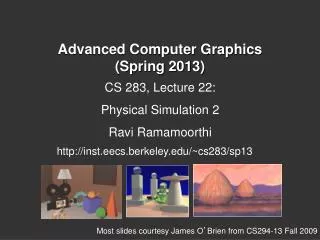
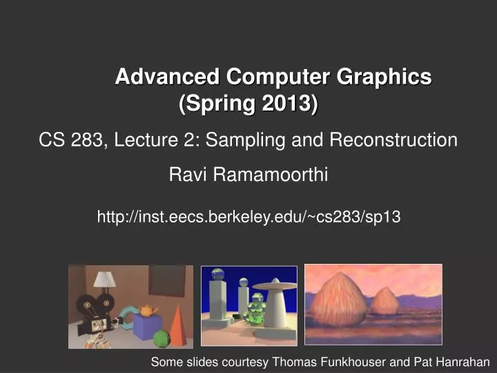
Advanced Computer Graphics (Spring 2013). CS 283, Lecture 2: Sampling and Reconstruction Ravi Ramamoorthi. http:// inst.eecs.berkeley.edu /~cs283 /sp13. Some slides courtesy Thomas Funkhouser and Pat Hanrahan. Basics. First 3 lectures cover basic topics

E N D
Advanced Computer Graphics (Spring 2013) CS 283, Lecture 2: Sampling and Reconstruction Ravi Ramamoorthi http://inst.eecs.berkeley.edu/~cs283/sp13 Some slides courtesy Thomas Funkhouser and Pat Hanrahan
Basics • First 3 lectures cover basic topics • Sampling and Reconstruction, Fourier Analysis • 3D objects and meshes • If you don’t know raytracing, look at online lectures, hw • Then we start main part of course • Meshes and assignment 1 • This lecture review for some of you • But needed to bring everyone up to speed • Much more detailed material available if interested (we have only limited time; cover it quickly) • Sign up for Piazza, E-mail Brandon re roster
Outline • Basic ideas of sampling, reconstruction, aliasing • Signal processing and Fourier analysis • Implementation of digital filters • Section 14.10 of FvDFH (you really should read) Some slides courtesy Tom Funkhouser
Sampling and Reconstruction • An image is a 2D array of samples • Discrete samples from real-world continuous signal
(Spatial) Aliasing • Jaggies probably biggest aliasing problem
Sampling and Aliasing • Artifacts due to undersampling or poor reconstruction • Formally, high frequencies masquerading as low • E.g. high frequency line as low freq jaggies
Outline • Basic ideas of sampling, reconstruction, aliasing • Signal processing and Fourier analysis • Implementation of digital filters • Section 14.10 of textbook
Motivation • Formal analysis of sampling and reconstruction • Important theory (signal-processing) for graphics • Also relevant in rendering, modeling, animation
Ideas • Signal (function of time generally, here of space) • Continuous: defined at all points; discrete: on a grid • High frequency: rapid variation; Low Freq: slow variation • Images are converting continuous to discrete. Do this sampling as best as possible. • Signal processing theory tells us how best to do this • Based on concept of frequency domain Fourier analysis
Sampling Theory Analysis in the frequency (not spatial) domain • Sum of sine waves, with possibly different offsets (phase) • Each wave different frequency, amplitude
Fourier Transform • Tool for converting from spatial to frequency domain • Or vice versa • One of most important mathematical ideas • Computational algorithm: Fast Fourier Transform • One of 10 great algorithms scientific computing • Makes Fourier processing possible (images etc.) • Not discussed here, but look up if interested
Fourier Transform • Simple case, function sum of sines, cosines • Continuous infinite case
Fourier Transform • Simple case, function sum of sines, cosines • Discrete case
Fourier Transform: Examples 1 • Single sine curve (+constant DC term)
Fourier Transform Examples 2 • Common examples
Fourier Transform Properties • Common properties • Linearity: • Derivatives: [integrate by parts] • 2D Fourier Transform • Convolution (next)
Sampling Theorem, Bandlimiting • A signal can be reconstructed from its samples, if the original signal has no frequencies above half the sampling frequency – Shannon • The minimum sampling rate for a bandlimited function is called the Nyquist rate
Sampling Theorem, Bandlimiting • A signal can be reconstructed from its samples, if the original signal has no frequencies above half the sampling frequency – Shannon • The minimum sampling rate for a bandlimited function is called the Nyquist rate • A signal is bandlimited if the highest frequency is bounded. This frequency is called the bandwidth • In general, when we transform, we want to filter to bandlimit before sampling, to avoid aliasing
Antialiasing • Sample at higher rate • Not always possible • Real world: lines have infinitely high frequencies, can’t sample at high enough resolution • Prefilter to bandlimit signal • Low-pass filtering (blurring) • Trade blurriness for aliasing
Ideal bandlimiting filter • Formal derivation is homework exercise
Outline • Basic ideas of sampling, reconstruction, aliasing • Signal processing and Fourier analysis • Convolution • Implementation of digital filters • Section 14.10 of FvDFH
Convolution in Frequency Domain • Convolution (f is signal ; g is filter [or vice versa]) • Fourier analysis (frequency domain multiplication)
Practical Image Processing • Discrete convolution (in spatial domain) with filters for various digital signal processing operations • Easy to analyze, understand effects in frequency domain • E.g. blurring or bandlimiting by convolving with low pass filter
Outline • Basic ideas of sampling, reconstruction, aliasing • Signal processing and Fourier analysis • Implementation of digital filters • Section 14.10 of FvDFH
Discrete Convolution • Previously: Convolution as mult in freq domain • But need to convert digital image to and from to use that • Useful in some cases, but not for small filters • Previously seen: Sinc as ideal low-pass filter • But has infinite spatial extent, exhibits spatial ringing • In general, use frequency ideas, but consider implementation issues as well • Instead, use simple discrete convolution filters e.g. • Pixel gets sum of nearby pixels weighted by filter/mask
Implementing Discrete Convolution • Fill in each pixel new image convolving with old • Not really possible to implement it in place • More efficient for smaller kernels/filters f • Normalization • If you don’t want overall brightness change, entries of filter must sum to 1. You may need to normalize by dividing • Integer arithmetic • Simpler and more efficient • In general, normalization outside, round to nearest int
Outline • Implementation of digital filters • Discrete convolution in spatial domain • Basic image-processing operations • Antialiased shift and resize
Basic Image Processing • Blur • Sharpen • Edge Detection All implemented using convolution with different filters
Blurring • Used for softening appearance • Convolve with gaussian filter • Same as mult. by gaussian in freq. domain, so reduces high-frequency content • Greater the spatial width, smaller the Fourier width, more blurring occurs and vice versa • How to find blurring filter?
Blurring Filter • In general, for symmetry f(u,v) = f(u) f(v) • You might want to have some fun with asymmetric filters • We will use a Gaussian blur • Blur width sigma depends on kernel size n (3,5,7,11,13,19) Frequency Spatial
Discrete Filtering, Normalization • Gaussian is infinite • In practice, finite filter of size n (much less energy beyond 2 sigma or 3 sigma). • Must renormalize so entries add up to 1 • Simple practical approach • Take smallest values as 1 to scale others, round to integers • Normalize. E.g. for n = 3, sigma = ½
Basic Image Processing • Blur • Sharpen • Edge Detection All implemented using convolution with different filters
Sharpening Filter • Unlike blur, want to accentuate high frequencies • Take differences with nearby pixels (rather than avg)
Basic Image Processing • Blur • Sharpen • Edge Detection All implemented using convolution with different filters