Materials Process Design and Control Laboratory

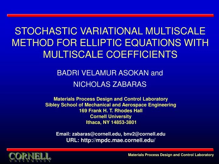
1. STOCHASTIC VARIATIONAL MULTISCALE METHOD FOR ELLIPTIC EQUATIONS WITH MULTISCALE COEFFICIENTS BADRI VELAMUR ASOKAN and NICHOLAS ZABARAS Materials Process Design and Control Laboratory Sibley School of Mechanical and Aerospace Engineering169 Frank H. T. Rhodes Hall Cornell University Ithaca, NY 14853-3801 Email: zabaras@cornell.edu, bnv2@cornell.edu URL: http://mpdc.mae.cornell.edu/

2. OUTLINE • Current techniques for multiscale elliptic equations • Variational multiscale [VMS] method • Generalized polynomial chaos approach • Deterministic VMS modeling of multiscale elliptic equation • Issues in extension of approach to stochastic elliptic equation • Presentation of subgrid problems • Numerical examples • Extensions to practical systems – A brief discussion

3. CURRENT TECHNIQUES • Stochastic VMS [Zabaras et al. JCP 208(1), 2005] • Residual-Free bubbles [Sangalli, SIAM MMS 1(3), 2003] • Adaptive variational multiscale method [Larson, Chalmers finite element preprints 2004-18, 2004-11] • Variational multiscale method [Arbogast, SIAM J.Num.Anal 42, 2004], [Arbogast, SPE J., Dec 2002] • Multiscale finite elements [Hou, JCP 134, 1997], [Hou, JCP, 2005] • Heterogeneous finite element method [Xu, J. Am. Math, 2003] • Homogenization and allied techniques

4. MODEL MULTISCALE ELLIPTIC EQUATION Boundary in on Domain • Multiple scale variations in K • K is inherently random [property predictions are at best statistical] Crystal microstructures • Composites • Diffusion processes Permeability of Upper Ness formation

5. STOCHASTIC PROCESSES AS FUNCTIONS • A probability space is a triple comprising of collection of basis outcomes , permutation of these outcomes and a probability measure • A real-valued random variable is a function that maps the probability space to a real line [regions in go to intervals in the real line] • : Random variable • A space-time stochastic process is can be represented as + other regularity conditions

6. SERIES REPRESENTATION [CONTD] • Karhunen-Loeve ON random variables Mean function Stochastic process Deterministic functions • Generalized polynomial chaos Stochastic input Askey polynomials in input Stochastic process Deterministic functions

7. STOCHASTIC VMS MODELING in on • K is spatially rapidly varying stochastic process [a multiscale diffusion coefficient] such that, for all [V] Find

8. Actual solution Subgrid scale solution Coarse scale solution h VARIATIONAL MULTISCALE METHOD • Hypothesis – Actual solution is a sum of coarse scale resolved part and a subgrid scale unresolved part [Hughes, 95] • This induces a similar decomposition of the governing equation into coarse and subgrid parts • Idea – Approximately solve the subgrid equations and include the effect on coarse scale equation • Highly successful with advection-diffusion problems, fluid-flow, micromechanics and other

9. VMS [VARIATIONAL FORMULATION] such that, for all [V] Find • [V] denotes the full variational formulation • U and V denote appropriate function spaces for the multiscale solution u and test function v respectively • VMS hypothesis: • Induced function space decomposition [Hughes 1995] Exact = coarse + fine

10. VMS [COARSE AND SUBGRID SCALES] and the induced function space Using decomposition Find and such that, for all and Coarse [V] Subgrid [V] • Solve subgrid [V] using Greens' functions, PU and other • Substitute the subgrid solution in coarse [V]

11. DEFINITIONS AND DISCRETIZATION • Since the subgrid solution uF represents rapid variations, more terms in GPCE is required • Let us now split the subgrid solution into two parts defined by the following equations Find and such that, for all and Subgrid [V] Homogeneous [V] Affine [V]

12. SOLUTION OF HOMOGENEOUS [V] Homogeneous [V] • This equation yields an approach similar to MsFEM technique for solving multiscale elliptic equations [Hou et al.] • By examination, is a map of the coarse solution on the subgrid scale • Since, represents subgrid variations, a higher order GPCE is used (leading to more terms in stochastic series expansion)

13. FINITE ELEMENT DISCRETIZATION Subgrid mesh • NelF elements • Associated with each element sub-domain in the coarse mesh Coarse mesh • NelC elements

14. DEFINITIONS AND DISCRETIZATION • Assume a finite element discretization of the spatial region D into NelC coarse elements • Each coarse element is further discretized by a subgrid mesh with NelF elements • In each coarse element, the coarse solution uC can be approximated as nbf= number of spatial finite element basis functions in each coarse element PC= number of terms in the GPCE of coarse solution

15. SOLUTION OF HOMOGENEOUS [V] CONTD • Considering the following finite element – GPCE representation for coarse solution uC • The subgrid solution can be represented as follows • Since represents subgrid variations, a nonlinear coarse scale mapping, a higher order GPCE is used [implies more terms in GPCE of ]

16. SOLUTION OF HOMOGENEOUS [V] CONTD • Now, we have • Thus, we end up with Nmax homogeneous subgrid problems in each coarse element D(e) • Following representation is used for approximation nbf= number of spatial finite element basis functions in each element defined on the subgrid mesh PF= number of terms in the GPCE. Also, PF >PC

17. HOMOGENEOUS [V] BOUNDARY CONDITIONS Coarse element D(e) • Also, reduced problems are solved on element sides for obtaining oscillatory boundary conditions Subgrid mesh

18. SOLVING REDUCED PROBLEM • Each coarse element edge is mapped to a line grid • Line grid yields coordinates (s – along the line grid, n – normal to line grid) • The reduced problem specified below is solved on the line grid Mapping element edge Subgrid mesh s n

19. FEM FOR HOMOGENEOUS [V] • Thus in each coarse element EC, we can solve for the subgrid basis functions as follows • Note that we solve for the sum of coarse + subgrid basis functions • The boundary conditions for this equation are obtained as the solution of the reduced problem on coarse element edges • DOF for the problem = (Nno-subgrid)(PF+1)

20. SOLUTION OF AFFINE [V] Affine [V] • This affine correction is unique to the VMS formulation [Arbogast et al.] and is not obtained in MsFEM type of formulations • Crucial in case of localized sources and sinks • Again, similar to the homogeneous [V], we have • This affine correction solution has no dependence on coarse scale behavior • We solve this equation on each coarse element with zero boundary conditions

21. DESCRIPTION OF NUMERICAL PROBLEMS Coarse element D(e) • Based on boundary conditions used and subgrid problems solved, we have three studies Subgrid mesh VMS-Os MsFEM-L MsFEM-Os • Reduced solution as BC • No affine correction • Reduced solution as BC • Affine correction explicitly solved • Linear boundary conditions are used • No affine correction

22. NUMERICAL EXAMPLES • Deterministic studies • Case 1: Periodic media [single fast scale separation] • Case 2: non-periodic media [multiple scales] • Stochastic studies • Case 1: Pseudo-periodic media • Effect of PF -PC difference • Future studies and research directions

23. DETERMINISTIC [CASE I] PERIODIC MEDIA • A 128x128 mesh for complete resolution • 4-noded bilinear quads for FEM K [periodic]

24. DETERMINISTIC [CASE I] RESULTS MsFEM-L Resolved FEM • coarse 8x8 subgrid 16x16 mesh • VMS yields consistent low error values MsFEM-Os VMS-Os

25. DETERMINISTIC [CASE II] NON-PERIODIC MEDIA • Presence of multiple spatial scales • non-periodic spatial variation • vertices v1(0,0) v2(1,0) v3(0,1) v4(1,1) K [non-periodic]

26. DETERMINISTIC [CASE II] NON-PERIODIC MEDIA • A 512x512 mesh for complete resolution • 4-noded bilinear quads for FEM

27. DETERMINISTIC [CASE II] RESULTS MsFEM-L Resolved FEM • coarse 16x16 subgrid 32x32 mesh • VMS yields consistent low error values MsFEM-Os VMS-Os

28. STOCHASTIC [CASE I] PSEUDO-PERIODIC MEDIA • uniformly distributed diffusion coefficient K0

29. DETERMINISTIC [CASE II] NON-PERIODIC MEDIA • A 512x512 mesh for complete resolution • 4-noded bilinear quads for FEM • MsFEM-L is not attempted owing to superior performance of MsFEM-Os and VMS-Os [for deterministic studies]

30. STOCHASTIC [CASE I] RESULTS VMS-Os FEM MsFEM-Os U0 U1 U2

31. STOCHASTIC [CASE I] ERROR MEASURES • L-inf error was calculated on the mean value • Again, VMS is consistently better than MsFEM-Os.

32. STOCHASTIC [CASE I] EFFECT OF PC TERMS • We have assumed that the fine scale solution has more PC terms in its expansion • While reconstructing the fully resolved solution from the fine scale solution, we can only reconstruct up to the PCC terms. Beyond those terms, the fine scale solution is no longer a one-to-one map, hence, we see abnormalities (still equal in L-2) L2 error Linf error PF-PC PF-PC

33. PRESENT AND FUTURE • Are currently applying VMS to transient diffusion problems in heterogeneous media • Applying VMS for solving convection-diffusion in random media • Implementation of over-sampling method in the context of VMS • Implementation of support-space techniques with VMS hypothesis applied in sample space [spatial and stochastic VMS] • Adaptive generation and solution of subgrid problems, specifically in convection-diffusion applications