Download
1 / 24
390 likes | 706 Vues
WRF-ARW Basics. Fundamentals of NWP Real vs. artificial atmosphere Map projections Horizontal grid staggering Vertical coordinate systems Definitions & Acronyms Flavors of WRF ARW core NMM core Other Numerical Weather Prediction Models MM5 ARPS Global Icosahedral

E N D
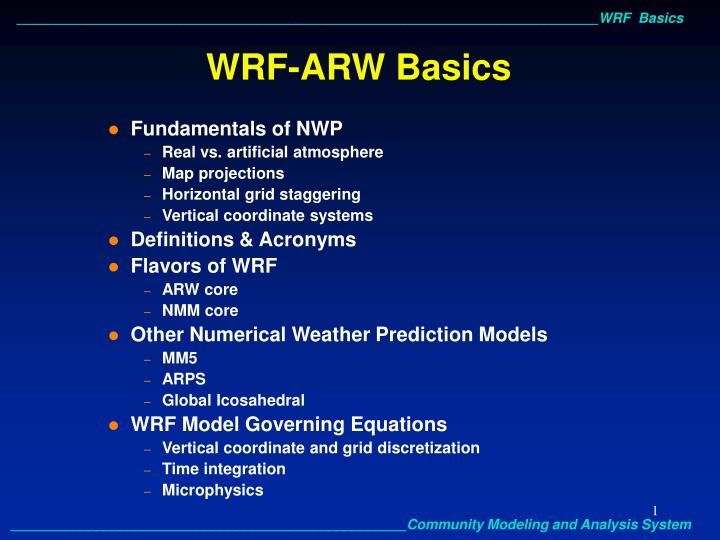
WRF-ARW Basics • Fundamentals of NWP • Real vs. artificial atmosphere • Map projections • Horizontal grid staggering • Vertical coordinate systems • Definitions & Acronyms • Flavors of WRF • ARW core • NMM core • Other Numerical Weather Prediction Models • MM5 • ARPS • Global Icosahedral • WRF Model Governing Equations • Vertical coordinate and grid discretization • Time integration • Microphysics
Real vs. Artificial Atmosphere True analytical solutions are unknown! Numerical models are discrete approximations of a continuous fluid.
Map Projections Example of a regional high resolution grid (projection of a spherical surface onto a 2D plane) nested within a global (lat,lon) grid with spherical coordinates x = r cos y = r Differences in map projections require caution when dealing with flow of information across grid boundaries. WRF offers polar stereographic, Lambert conformal, Mercator and rotated Lat-Lon map projections.
Arakawa “A” Grid • Unstaggered grid - all variables defined everywhere. • Poor performance, first grid geometry employed in NWP models. • Can use a 2x larger time step than staggered grids. • Noisy - large errors, short waves propagate energy in wrong direction, additional smoothing required. • Poorest at geostrophic adjustment - wave energy trapped, heights remain too high.
Arakawa “B” Grid • Staggered, velocity at corners. • Preferred at coarse resolution. • Superior for poorly resolved inertia-gravity waves. • Good for geostrophy, Rossby waves: collocation of velocity points. • Bad for gravity waves: computational checkerboard mode. • Used by MM5 model.
Arakawa “C” Grid • Staggered, mass at center, normal velocity, fluxes at grid cell faces, vorticity at corners. • Preferred at fine resolution. • Superior for gravity waves. • Good for well resolved inertia-gravity waves. • Simulates Kelvin waves (shoulder on boundary) well. • Bad for poorly resolved waves: Rossby waves (computational checkerboard mode) and inertia-gravity waves due to averaging the Coriolis force. • Used by WRF-ARW, ARPS, CMAQ models.
Arakawa “D” Grid • Staggered, mass at center, tangential velocity along grid faces. • Poorest performance, worst dispersion properties, rarely used. • Noisy - large errors, short waves propagate energy in wrong direction.
Arakawa “E” Grid • Semi-staggered grid. • Equivalent to superposition of 2 C-grids, then rotated 45 degrees. • Center set to translated (lat,lon) = (0,0) to prevent distortion near edges, poles. • Developed for Eta step-mountain coordinate to enhance blocking, overcome PGF errors caused by sigma coordinates. • Controls the cascade of energy toward smaller scales. • Used by WRF-NMM and Eta models.
Definitions & Acronyms • WRF: Weather Research & Forecasting numerical weather prediction model • ARW: Advanced Research WRF [nee Eulerian Model (EM)] core • NMM: Nonhydrostatic Mesoscale Model core • WRF-SI: Standard Initialization (4 components) - prepares real atmospheric data for input to WRF • WRF-VAR: Variational 3D/4D data assimilation system (not used for this class) • IDV: Integrated Data Viewer - Java application for interactive visualization of WRF model output
Flavors of WRF (ARW) • ARW solver (research - NCAR, Boulder, Colorado) • Fully compressible, nonhydrostatic equations with hydrostatic option • Arakawa-C horizontal grid staggering • Mass-based terrain following vertical coordinate • Vertical grid spacing can vary with height • Top is a constant pressure surface • Scalar-conserving flux form for prognostic model variables • 2nd to 6th-order advection options in horizontal &vertical • One-way, two-way and movable nest options • Runge-Kutta 2nd & 3rd-order time integration options • Time-splitting • Large time step for advection • Small time step for acoustic and internal gravity waves • Small step horizontally explicit, vertically implicit • Divergence damping for suppressing sound waves • Full physics options for land surface, PBL, radiation, microphysics and cumulus parameterization • WRF-chem under development: http://ruc.fsl.noaa.gov/wrf/WG11/
Flavors of WRF (NMM) • NMM solver (operational - NCEP, Camp Springs, Maryland) • Fully compressible, nonhydrostatic equations with reduced hydrostatic option • Arakawa-E horizontal grid staggering, rotated latitude-longitude • Hybrid sigma-pressure vertical coordinate • Conservative, positive definite, flux-corrected scheme used for horizontal and vertical advection of TKE and water species • 2nd-order spatial that conserves a number of 1st-order and quadratic quantities, including energy and enstrophy • One-way, two-way and movable nesting options • Time-integration schemes: forward-backward for horizontally propagating fast waves, implicit for vertically propagating sound waves, Adams-Bashforth for horizontal advection and Coriolis force, and Crank-Nicholson for vertical advection • Divergence damping & E subgrid coupling for suppressing sound waves • Full physics options for land surface, PBL, radiation, microphysics (only Ferrier scheme) and cumulus parameterization • Note: Many ARW core options are not yet implemented! Nesting still under development • NMM core will be used for HWRF (hurricane version of WRF), operational in summer of 2007
Other NWP Models (MM5) • MM5 (research - PSU/NCAR, Boulder, Colorado) • Progenitor of WRF-ARW, mature NWP model with extensive configuration options • Support terminated, no future enhancements by NCAR’s MMM division • Nonhydrostatic and hydrostatic frameworks • Arakawa-B horizontal grid staggering • Terrain following sigma vertical coordinate • Unsophisticated advective transport schemes cause dispersion, dissipation, poor mass conservation, lack of shape preservation • Outdated Leapfrog time integration scheme • One-way and two-way (including movable) nesting options • 4-dimensional data assimilation via nudging (Newtonian relaxation), 3D-VAR, and adjoint model • Full physics options for land surface, PBL, radiation, microphysics and cumulus parameterization
Other NWP Models (ARPS) • ARPS (research - CAPS/OU, Norman, Oklahoma) • Advanced Regional Prediction System • Sophisticated NWP model with capabilities similar to WRF • Primarily used for tornado simulations and assimilation of experimental radar data at mesoscale and ultra-high (25 meter) resolutions • Elegant, source code, easy to read/understand/modify, ideal for research projects, very helpful scientists at CAPS • Arakawa-C horizontal grid staggering • Currently lacks full mass conservation and Runge-Kutta time integration scheme • ARPS Data Assimilation System (ADAS) under active development/enhancement (MPI version soon), faster & more flexible than WRF-SI, employed in LEAD NSF cyber-infrastructure project • wrf2arps and arps2wrf data set conversion programs available • http://www.caps.ou.edu/ARPS/arpsdownload.html
WRF Model Governing Equations(Eulerian Flux Form) Momentum: ∂U/∂t + (∇ · Vu) − ∂(pφη)/∂x + ∂(pφx)/∂η = FU ∂V/∂t + (∇ · Vv) − ∂(pφη)/∂y + ∂(pφy)/∂η = FV ∂W/∂t + (∇ · Vw) − g(∂p/∂η − μ) = FW Potential Temperature: Inverse Density (): ∂Θ/∂t + (∇ · Vθ) = FΘ ∂φ/∂η = -μ Continuity: where: μ = column mass V = μv = (U,V,W) Ω = μ d(η)/dt Θ = μθ ∂μ/∂t + (∇ · V) = 0 Geopotential Height: ∂φ/∂t + μ−1[(V · ∇φ) − gW] = 0
Square Wave Advection Tests Φ∗ = Φt + t/3 R(Φt ) Φ∗∗ = Φt + t/2 R(Φ∗) Φt+t = Φt + t R(Φ∗∗)
Runge-Kutta Time Step Constraint • RK3 is limited by the advective Courant number (ut/x) and the user’s choice of advection schemes (2nd through 6th order) • The maximum stable Courant numbers for advection in the RK3 scheme are almost double those in the leapfrog time-integration scheme Maximum Courant number for 1D advection in RK3
Microphysics • Includes explicitly resolved water vapor, cloud and precipitation processes • Model accommodates any number of mixing-ratio variables • Four-dimensional arrays with 3 spatial indices and one species index • Memory (size of 4th dimension) is allocated depending on the scheme • Carried out at the end of the time-step as an adjustment process, does not provide tendencies • Rationale: condensation adjustment should be at the end of the time step to guarantee that the final saturation balance is accurate for the updated temperature and moisture • Latent heating forcing for potential temperature during dynamical sub-steps (saving the microphysical heating as an approximation for the next time step) • Sedimentation process is accounted for, a smaller time step is allowed to calculate vertical flux of precipitation to prevent instability • Saturation adjustment is also included
WRF Microphysics Options • Mixed-phase processes are those that result from the interaction of ice and water particles (e.g. riming that produces graupel or hail) • For grid sizes ≤ 10 km, where updrafts may be resolved, mixed-phase schemes should be used, particularly in convective or icing situations • For coarser grids the added expense of these schemes is not worth it because riming is not likely to be resolved