Download
1 / 17
190 likes | 406 Vues
EVALUATING WRF- arw v3.4.1 simulations of tropical cyclone yasi. Chelsea Parker, Amanda Lynch, Maria Tsukernik (Brown University) , Todd Arbetter (CRREL) 14 th Annual WRF User’s Workshop Thursday June 27 th 2013. Outline. Background of Case Study Tropical Cyclone Yasi

E N D
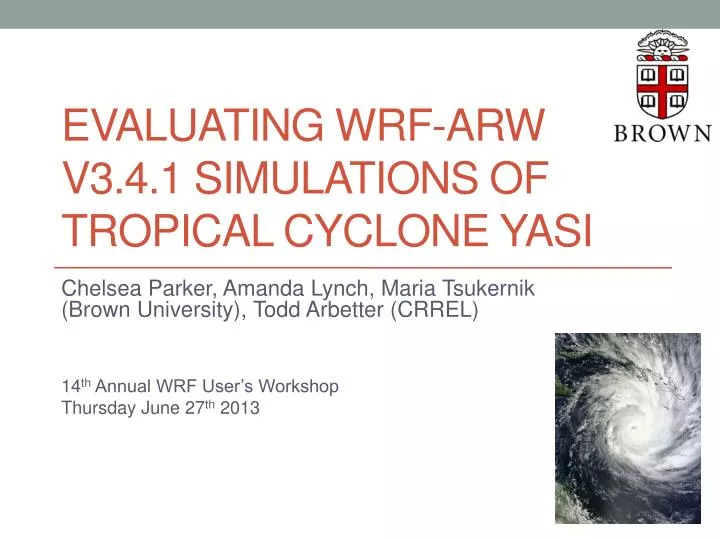
EVALUATING WRF-arw v3.4.1 simulations of tropical cyclone yasi Chelsea Parker, Amanda Lynch, Maria Tsukernik(Brown University), Todd Arbetter (CRREL) 14th Annual WRF User’s Workshop Thursday June 27th 2013
Outline • Background of Case Study Tropical Cyclone Yasi • WRF v3.4.1 model set up • Physics Sensitivity Simulations • Results and Analysis • Conclusions
YASI Rapidly intensifying, category 5 storm. Cyclogenesisnortheastof Fiji on 29thJan, landfall on the Queensland coastline in early hours Feb 3rd 2011. 600km wide, eye 35km wide. 6m storm surge. Wind speed up to 300 km/h. 929hPa minimum low Wunderground.com
LIFE CYCLE YASI 2011 CYCLONE SEASON Australian Bureau of Meteorology, 2011 Australian Bureau of Meteorology, 2011
MODEL SET UP d01, 36km d02, 12km d03, 4km 27 vertical levels ptop: 50hPa 4day simulations from Jan 31st 00:00 to Feb 4th 2011 00:00 UTC. Shortwave: Dudhia Longwave: RRTM Surface layer: MM5 Monin-Obukhov Land surface: Unified Noah LSM
INITIALISATION and FORCING DATA ERA INTERIM Reanalysis data, ~80km resolution Bureau of Meteorology Initialisation, 4km resolution
Physics package trials • Cumulus parameter (CU): • Microphysics (MP): • Planetary Boundary Layer (PBL): • ISFTCFLX: off or with 2, Donelan Cd + Garrett scheme • OMLCALL: off or with 50m 1D simple ocean mixed layer. (Land Surface: Thermal Diffusion Scheme)
Simulated TC Tracks Track Colour key: Black = Cu = 0 None Green: Cu = 1 K-F Yellow: Cu=2 BMJ Cyan: Cu = 3 G-D Blue: Cu=5 Grell 3D Red: Cu=6 Tiedtke Runs with CU 6 cluster the most throughout the whole simulation even after landfall and get the closest to the correct landfall location. Runs with CU 1 show the most southerly motion of the track and the greatest deviation from the landfall location. Wikipedia.org
ERA Default ERABOM Default CU2MP4PBL1 CU1MP5PBL1 CU3MP5PBL1 CU5MP5PBL1 CU6MP5PBL1 CU6MP6PBL1 CU6MP6PBL1 ISFLX CU6MP6PBL1 ISFLX OML CU1MP6PBL1 CU1MP6PBL1 ISFLX CU1MP6PBL1 ISFLX OML CU1MP6PBL5 ISFLX OML CU2MP1PBL1 ISFLX OML CU6MP5PBL1 ISFLX CU6MP5PBL1 ISFLX CU6MP5PBL5 ISFLX OML CU6MP6PBL5 ISFLX OML CU6MP4PBL1 Normalised Root-Mean-Square Error Index:Landfall location, timing and central pressure
Statistical ANOVA test Coefficients: Estimate Std.Error t value Pr(>|t|) (Intercept) 1.103 0.071 15.600 3.02e-10 *** YASI$CU -0.074 0.012 -6.150 2.52e-05 *** YASI$MP -0.037 0.017 -2.192 0.046 * YASI$PBL -0.002 0.024 -0.089 0.930 YASI$ISFLX 0.082 0.082 0.999 0.335 YASI$OML -0.017 0.093 -0.187 0.854 --- Signif. codes: 0 ‘***’ 0.001 ‘**’ 0.01 ‘*’ 0.05 ‘.’ 0.1 ‘ ’ 1 Residual standard error: 0.1181 on 14 degrees of freedom Multiple R-squared: 0.8251, Adjusted R-squared: 0.7626 F-statistic: 13.21 on 5 and 14 DF, p-value: 6.947e-05 • All the components account for ~76% of variance in the calculated error index and this is statistically significant. • Variance in CU parameter individually is statistically significant in predicting the error index variance. • Changing MP parameter also individually affects the variance of the error index but to a lesser significance. • None of the other physics parameters have a statistically significant relationship with predicting the error index individually.
SLP and Track CU 1 K-F more accurate minimum sea level pressure (SLP) values and evolution of values and therefore intensity. CU 6Tiedtke more accurate track evolution and landfall location. For almost all runs, the minimum in SLP occurs over the open ocean around 08:00 1st Feb 2011 UTC which is too early and then weaken towards landfall. Wikipedia.org CU6MP5PBL1 CU1MP5PBL1
WRF Output: Total Accumulated Precipitation, Tiedtke-WSM 6-YSU Earthobservatory.nasa.gov
Conclusions • Prescribing physics parameters key in improving the accuracy of the simulated TC Yasi and reducing the calculated error. • Cumulus parameter had the biggest effect on altering the produced TC and the calculated error index by affecting the pressure, timing and location of the TC throughout the lifecycle and especially at landfall. • Kain-Fritsch scheme produces a closest to accurate simulation of pressure and landfall timing but the greatest deviation of distance. Modified Tiedtke scheme produces the most accurate track. • ‘Best’ simulations according to the error index use Modified Tiedtke-Ferrier-YSU or when implementing ISFTCFLX and OML then Modified Tiedtke-WSM6-YSU • Still problems with TC life cycle simulation even in these ‘best’ cases. • Still more schemes to test such as Thompson MP scheme and other PBL schemes and other output parameters and differences to consider.
Acknowledgements • Amanda Lynch, Masha Tsukernik, Henry Johnson (Brown University). • Todd Arbetter (CRREL) • Noel Davidson (Bureau of Meteorology, Australia) Thank You!
Wind Shear, Warm Advection, Latent and Sensible Heat Fluxes CU1 MP5 PBL1 CU6 MP5 PBL1
Next Steps • Also consider size and wind fields in skill score. • Further analyse the output from the physics trials particularly for wind shear, warm advection, latent and sensible heat. • Choose the most appropriate simulation and its physics combination to move forward. • Add a high resolution sea surface temperature (SST) field in to the WRF simulation to see how TC Yasi changes. • Further test the TC’s sensitivity to SST by manually altering the SST magnitudes and gradients across the western South Pacific in the vicinity of Yasi’s track. • ROMS? COAWST?