Download
1 / 13
170 likes | 408 Vues
Introduction Monday 21 st 9-10am Turbulence theory Monday 21 st 11-12am Measuring turbulence Monday 28 th 9-10am Modelling turbulence Monday 28 th 11-12am . Marine Turbulence and Mixing. 2. Turbulence theory. Dr. Matthew Palmer matthew.palmer@noc.ac.uk.

E N D
Introduction Monday 21st 9-10am Turbulence theory Monday 21st 11-12am Measuring turbulence Monday 28th 9-10am Modelling turbulence Monday 28th 11-12am Marine Turbulence and Mixing 2. Turbulence theory Dr. Matthew Palmer matthew.palmer@noc.ac.uk
Definition of turbulence: • Random, chaotic, irregular and unpredictable. Requires statistical representation. • Vortical. • 3-dimensional. • Dissipative, always. • Unsteady, unstable. Occurring over a broad spectrum of length and time scales. • Diffusive. Promoting enhanced transfer by mixing.
A statistical representation of turbulence • Turbulence is complex, chaotic and unstable • It is therefore impossible to predict • A convenient method of describing turbulence separates the flow u into the predictable mean part U and the turbulent part u’. • We refer to this technique as Reynolds decomposition. Osbourne Reynolds 1842 -1912 U u = U + u’
Representing turbulence in the equations of motion W+w’ z w v V+v’ Consider the momentum flux (unit area) in the x direction of a particle through area A at the velocity u, or U+u’. y U+u’ u = x A Momentum flux = (mass(m-3) x velocity) x flux through A r (u+u’).(u+u’).A The mean force per unit area, or stress, in the x direction by flow u is, and in the y and z direction, r (U+u’).(V+v’).A r (U+u’).(W+w’).A and but , so
Normal stresses Symmetric In the ocean, vertical gradients are much stronger than horizontal so we may disregard horizontal components of stress The 9 cartesian Reynolds stress tensor So we may now only consider txz and tyz or r u’w’ and r v’w’ u' z w' x Reynolds decomposition is also applicable to scalar quantities (temperature, salinity, density, nutrients etc.) s = S + s’ s‘ = 0
Parameterisation of turbulence But remember, turbulence is random, chaotic, broad spectrum and so difficult to measure. So we often need to parameterise the process of generating turbulence. Consider how turbulent eddies interact. Reynolds stress transfers energy from the horizontal to vertical and vortical turbulent motion. txz = r u’w’ tyz = r v’w’ Sheared Flow Due to its diffusive nature we may approximate these stresses to act in a similar way to molecular diffusivity but on larger scales (Bousinesq). We may then parameterise the generation of turbulence by gradients in the mean flow. 1842-1929 Nz is the vertical eddy viscosity coefficient (m2s-1)
Introducing eddy diffusivity: Remember that we may consider the turbulent properties of scalar quantities such as density or temperature in the same was as momentum. s = S + s’ s‘ = 0 We may also approximate eddy diffusivity from molecular processes. therfore Kz is the vertical eddy diffusivity coefficient (m2s-1) Which gives us the advection-diffusion equation for a scalar quantity: Which represents the local rate of change of the scalar s in terms of horizontal advection by the mean flow U and vertical diffusion by the turbulent fluctuations within the water column.
EoM and the TKE budget: We now have methods for quantifying complex turbulent processes by representing the statistical properties of turbulent flow and by considering them to behave similar to molecular processes, within the equations of motion and within the turbulent kinetic energy (E) budget, Where P = production (+ve) B = buoyant production (+ve or –ve) e = dissipation (-ve)
A solution for Kz In the absence of convection, there is TKE production is in balance with work against buoyancy and TKE dissipation. e Buoyant P But there is a limiting factor! Above a certain ratio of B/P turbulence will be suppressed. Production So we can define an expression to calculate the eddy diffusivity coefficient Kz. Where Where G ~0.2 (Osborn, 1980)
Instability and the transition to turbulence: introducing the gradient Richardson number Rig If velocity changes with depth in a stable, stratified flow, then the flow may become unstable providing that the shear flow is large enough. The limiting condition for the development of turbulence is that the energy supply from the mean flow is greater than the energy demands of dissipation and mixing. Turbulence is hungry! Assuming that NzKz, then we may consider the relative stability as a competition between destabilising shear flow and stabilising buoyancy. The gradient Richardson number, Where Rig ≤ ¼ somewhere within the flow instability may exist and disturbances may grow (Miles (1961) and Howard (1961) )
Summary: • Turbulent properties are chaotic so difficult to quantify. • We have therefore represented turbulence in the EoM by approximation of its statistical properties. • Using Nz and Kz to represent the viscous and diffusive nature of turbulence. • Defined an expression for turbulent diffusion, Kz. • Provided a method for quantifying the relative stability of the flow using Rig.
Acoustic Doppler Current Profiler (ADCP) ADCPs are able to sample u fast enough to measure u’w’ and v’w’ and so we can directly calculate Reynolds stresses, eddy viscosity and TKE production…… …..Next week