Download
1 / 13
140 likes | 315 Vues
Introduction Monday 21 st 9-10am Turbulence theory Monday 21 st 11-12am Measuring turbulence Monday 28 th 9-10am Modelling turbulence Monday 28 th 11-12am . Marine Turbulence and Mixing. 3 . Measuring turbulence. Dr. Matthew Palmer matthew.palmer@noc.ac.uk.

E N D
Introduction Monday 21st 9-10am Turbulence theory Monday 21st 11-12am Measuring turbulence Monday 28th 9-10am Modelling turbulence Monday 28th 11-12am Marine Turbulence and Mixing 3. Measuring turbulence Dr. Matthew Palmer matthew.palmer@noc.ac.uk
Summary from last week: • Turbulent mixing in ocean underpins many of the critical components in our Earth system. • There are numerous sources of mixing, however the mechanisms that lead to mixing are generally similar. • And although ‘chaotic’, turbulence exhibits recognisable characteristics. • We may characterise the static state of our oceans by the amount of energy required to mix the water column. (J m-2) Shear driven instability
Summary from last week: • Turbulent properties are chaotic so difficult to quantify. • We have therefore represented turbulence in the EoM by approximation of its statistical properties. • Using Nz and Kz to represent the viscous and diffusive nature of turbulence. • Defined an expression for turbulent diffusion, Kz. • Provided a method for quantifying the relative stability of the flow using Rig.
Measuring marine turbulence and quantifying mixing: • Change of state with time, consider the PE within a system and how it changes. • But this represents an integrated perspective... • ...and is a static solution, what about advection? Or propagating energy? • So we wish to measure turbulence directly so we can estimate turbulent mixing.
Turbulent length scales: • Consider the largest possible turbulent length scales to be ~width of the sheared flow, L. • Energy is extracted from large eddies to eddies of ever decreasing size through a process of vortex stretching. • Small eddies will not interact with larger eddies or the mean flow, remember u’=0. • So energy is passed down an irreversible inertial cascade to ever decreasing length scales. • But since angular momentum is conserved, velocity gradients will become stronger and stronger until viscosity smears out velocity fluctuations (u’) and energy is final dissipated as heat. Big Whorls Have Little Whorls Big whorls have little whorls That feed on their velocity, And little whorls have lesser whorls And so on to viscosity. 1881-1953 1881-1953 Lewis Fry Richardson
Turbulent length scales: 1903-1907 Andrey Kolmogorov 1903-1987 Andrey Kolmogorov • Kolmogorov postulated that the smallest ‘dissipative’ length scale, or microscale, (h) is dependent only on the rate of dissipation of turbulent kinetic energy (e) and kinematic viscosity (u). • uvarys little, ~1-2 x 10⁻⁶ m2s-1 in 0-20oC seawater. (m) • Highly turbulent regimes e.g. Near bed, e O[10-3Wkg-1] • In low energy regimes e.g. pycnocline, e O[10-8Wkg-1] • So h typically ranges from O[0.1mm] to O[10mm] over the whole ocean Dissipation to heat The cascade of energy from the largest turbulent eddy to the Kolmogorov microscale is termed the inertial subrange; =h The cascade of energy from large to small scales by the process of vortex stretching. The integral of S represents the total amount of energy dissipated, e.
Measuring turbulent spectra and e with shear microstructure This method depends on highly sensitive piezo-electric probes that produce a variable voltage relative to the lateral flow, or shear, across the probe • Turbulent Microstructure Profiler: • Profiles are typically collected during the descent from the aft of a ship or platform. • but can be upward profiling for near surface measurements, or autonomous for deep ocean. • Fall rates 0.4 – 0.8 ms-1 (with similar ascent) • So a single cast in 100m of water takes 250-500s • Other sensors measure temperature, salinity, pressure etc. u'
Turbulent Microstructure Profiler: • Not all of the inertial sub-range can be captured • limited by the size of the profiler, • the size of the probe tip, • and instrument noise, both electronic and mechanical. • collision with suspended matter/biology. • The predictable cascade of energy however permits us to estimate the missing components of the energy spectrum1. As the profiler descends, the probes interact with the range of turbulent eddies within the inertial sub-range. The dissipation rate of TKE, , can then be derived from the variance of the shear- Where m = kinematic viscosity of sea water, Noise
Turbulence measured using acoustic methods: ADCPs f0 • Acoustic Doppler Current Profiler transducers transmit (A) acoustic pulses and receive (B) the backscattered signal. • The relative velocity (V) of suspended particles is proportional to the ‘Doppler shift’ of the returned frequency (fD) of the original acoustic signal (f0). fD c = speed of sound in seawater~1500ms-1
ADCP: 3-D current vectors Converting radial velocity to Cartesian coordinates • ADCPs typically use 4 beams in a ‘Janus’ configuration separated by 20o angles from the vertical axis. • Each beam (i = 1 to 4) only records radial (along beam) velocity (bi)which is a combination of each of its Cartesian components u, v and w. • If we assume stationarity between opposite beams, i.e. they see the same packet of water/similarly behaving water, • then we can use basic trigonometry to derive horizontal and vertical velocity: u, v and w. • To calculate current velocity at different ranges, or bins, from the transducer to produce a current velocity profile. j1Heading j2 Pitch j3 Roll Problem: turbulent flows are unlikely to satisfy stationarity over large distances (>L)
ADCP: Reynolds stress and TKE production • If we can measure the variance of the radial velocity (which contains both (u’ and w’ components) we can directly measure Reynolds stress. • And combined with the vertical shear in the mean flow U…. • Estimate the production rate of TKE, P
Understanding turbulence through measurements of Nz and Kz • So we can now make characterise the bulk properties of a turbulent flow. • How turbulence is transferred through a sheared flow and dissipated, via the eddy viscosity coefficient Nz. • And how that energy mixes vertical gradients, via the eddy viscosity coefficient Kz.
Summary • Turbulence dissipates in an irreversible inertial cascade, described by Kolmogorov and verified with measurements by Nasmyth. • This permits is to estimate the dissipation rate of TKE, e, by integration of the shear microstructure within the inertial subrange. • Through acoustic methods we are able to measure the mean and turbulent components of flow, U and u’. • We can therefore calculate the mean vertical shear dU/dz and Reynolds stress u’w’, and derive the production rate of TKE, P and the eddy viscosity, Nz. • From e we are able to calculate the turbulent diffusion rate Kz. • We will now see how these values are represented and calculated in models…..