Download
1 / 64
1.45k likes | 4.53k Vues
Capacitance and Laplace’s Equation. Capacitance Definition Simple Capacitance Examples Capacitance Example using Streamlines & Images Two-wire Transmission Line Conducting Cylinder/Plane Field Sketching Laplace and Poison’s Equation Laplace’s Equation Examples

E N D
Capacitance and Laplace’s Equation • Capacitance Definition • Simple Capacitance Examples • Capacitance Example using Streamlines & Images • Two-wire Transmission Line • Conducting Cylinder/Plane • Field Sketching • Laplace and Poison’s Equation • Laplace’s Equation Examples • Laplace’s Equation - Separation of variables • Poisson’s Equation Example
Potential of various charge arrangements • Point • Line (coaxial) • Sheet • V proportional to Q, with some factor involving geometry • Define
A simple capacitor consists of two oppositely charged conductors surrounded by a uniform dielectric. An increase in Q by some factor results in an increase D (and E) by same factor. With the potential difference between conductors: S Q . A increasing by the same factor -- so the ratio Q to V0 is constant. We define the capacitance of the structure as the ratio of stored charge to applied voltage, or E, D . -Q B Units are Coul/V or Farads Basic Capacitance Definition
The horizontal dimensions are assumed to be much greater than the plate separation, d. The electric field thus lies only in the z direction, with the potential varying only with z. Plate area = S Applying boundary conditions for D at surface of a perfect conductor: Lower plate: Same result either way! Upper Plate: Boundary conditions needed at only onesurface to obtain total field between plates. Electric field between plates is therefore: Example 1 - Parallel-Plate Capacitor - I
With Electric Field Plate area = S The voltage between plates is: Combining with capacitance is Example 1 - Parallel-Plate Capacitor - II Note In region between plates
Stored energy is found by integrating the energy density in the electric field over the capacitor volume. Rearranging gives S V02 C Gives 3 ways of stored energy: Energy Stored in parallel-plate Capacitor From Chapter 4 page 102
Coaxial Electric Field using Gauss’ Law: S E 1 assume a unit length in z E = 0 elsewhere, assuming hollow inner conductor, equal and opposite charges on inner and outer conductors. Example 2 - Coaxial Transmission Line - I Writing with surface-charge density Simplifying
Electric Field between conductors S Potential difference between conductors: E 1 assume unit length in z Charge per unit length on inner conductor Gives capacitance: Example 2 - Coaxial Transmission Line - II
Two concentric spherical conductors of radii a and b, with equal and opposite charges Q on inner and outer conductors. From Gauss’ Law, electric field exists only between spheres and is given by: E a -Q Q b Potential difference between inner and outer spheres is Capacitance is thus: Note as (isolated sphere) Example 3 – Concentric Spherical Capacitor
A conducting sphere of radius a carries charge Q. A dielectric layer of thickness (r1 – a)and of permittivity 1surrounds the conductor. Electric field in the 2 regions is found from Gauss’ Law a E2 Q E1 r1 The potential at the sphere surface (relative to infinity) is: = V0 The capacitance is: Example 4 - Sphere with Dielectric Coating
Surface charge on either plate is normal displacement DNthrough both dielectrics: Potential between top and bottom surfaces << Rule for 2 capacitors in series Example 5 – Parallel Capacitor with 2-Layer Dielectric The capacitance is thus:
y V = 0 V = V0 . b l x h a Example 6Two Parallel Wires vs. Conducting-Cylinder/Plane • Parallel wires on left substitute conducting cylinder/plane on right • Equipotential streamline for wires on left match equipotential surface for cylinder on right. • Image wire (-a) on left emulates vertical conducting plane on right. Two parallel wires Conducting cylinder/plane
Example 6 - Two Parallel Wires and Conducting-Cylinder/Plane • Parallel Wires • Superimpose 2 long-wire potentials at x = +a and x = -a. • Translate to common rectangular coordinate system. • Define parameter K (=constant) for V (=constant) equipotential. • Find streamlines (x,y) for constant K and constant V. • Conducting-Cylinder/Plane • Insert metal cylinder along equipotential (constant K) streamline. • Work backward to find long-wire position, charge density, and K parameter from cylinder diameter, offset, and V potential. • Calculate capacitance of cylinder/plane from long-wire position and charge density • Write expression for potential, D, and E fields between cylinder and plane. • Write expression for surface charge density on plane.
Begin with potential of single line charge on z axis, with zero reference at = R0 Then write potential for 2 line charges of opposite sign positioned at x = +a and x = -a Two Parallel Wires – Basic Potential
2 line charges of opposite sign: 2 Parallel Wires – Rectangular Coordinates Choose a common reference radius R10 = R20 . Write R1 and R2 in terms of common rectangular coordinates x, y.
2Parallel Wires – Using Parameter K Two opposite line charges in rectangular coordinates : Write ln( ) term as parameter K1: Corresponding to potential V = V1 according to: Corresponding to equipotential surface V = V1 for dimensionless parameter K = K1
2 Parallel Wires – Getting Streamlines for K Find streamlines for constant parameter K1 where voltage is constant V1 To better identify surface, expand the squares, and collect terms: y V = 0 V = V0 b l x h a Equation of circle (cylinder) with radius b and displaced along x axis h
2 Parallel Wires - Substituting Conducting-Cylinder/Plane Find physical parameters of wires (a, ρL, K1) from streamline parameters (h, b, Vo) and y Eliminate a in h and b equations to get quadratic V = 0 V = V0 Solution gives K parameter as function of cylinder diameter/offset b l x h a Choose positive sign for positive value for a Substitution above gives image wire position as function of cylinder diameter/offset
Equivalent line chargel for conducting cylinder is located at y From original definition or V = 0 Capacitance for length L is thus V = V0 . b l x h a Getting Capacitance of Conducting-Cylinder/Plane
Conducting cylinder radius b = 5 mm, offset h = 13 mm, potential V0= 100 V. Find offset of equivalent line charge a, parameter K, charge density l, and capacitance C. y mm V = 0 V = V0 . b l Charge density and capacitance x h a Results unchanged so long as relative proportions maintained Example 1 - Conducting Cylinder/Plane
For V0 = 50-volt equipotential surface we recalculate cylinder radius and offset mm mm The resulting surface is the dashed red circle Example 2 - Conducting Cylinder/Plane
Getting Fields for Conducting Cylinder/Plane • Gradient of Potential • Electric Field • Displacement • For original 5 mm cylinder diameter, 13 mm offset, and 12 mm image-wire offset • Where max and min are between cylinder and ground plane, and opposite ground plane y V = 0 V = V0 b l x h a
With two wires or cylinders (and zero potential plane between them) the structure represents two wire/plane or two cylinder/plane capacitors in series, so the overall capacitance is half that derived previously. b x h Finally, if the cylinder (wire) dimensions are much less than their spacing (b << h), then L Getting Capacitance of 2-Wire or 2-Cylinder Line
This method employs these properties of conductors and fields: Using Field Sketches to Estimate Capacitance
Given the conductor boundaries, equipotentials may be sketched in. An attempt is made to establish approximately equal potential differences between them. A line of electric flux density, D, is then started (at point A), and then drawn such that it crosses equipotential lines at right-angles. Sketching Equipotentials
Total Capacitance as # of Flux/Voltage Increments For conductor boundaries on left and right, capacitance is Writing with # flux increments and # voltage increments Electrode Electrode
Capacitance of Individual Flux/Voltage Increments Writing flux increment as flux density times area (1 m depth into page) Writing voltage increment as Electric field times distance Forming ratio
Total Capacitance for Square Flux/Voltage Increments Capacitance between conductor boundaries Combining with flux/voltage ratio Provided ΔLQ = ΔLV (increments square)
Laplace and Poisson’s Equation • Assert the obvious • Laplace - Flux must have zero divergence in empty space, consistent with geometry (rectangular, cylindrical, spherical) • Poisson - Flux divergence must be related to free charge density • This provides general form of potential and field with unknown integration constants. • Fit boundary conditions to find integration constants.
These equations allow one to find the potential field in a region, in which values of potential or electric field are known at its boundaries. Start with Maxwell’s first equation: where and so that or finally: Derivation of Poisson’s and Laplace’s Equations
Recall the divergence as expressed in rectangular coordinates: …and the gradient: then: It is known as the Laplacian operator . Poisson’s and Laplace’s Equations (continued)
we already have: which becomes: This is Poisson’s equation, as stated in rectangular coordinates. In the event that there is zero volume charge density, the right-hand-side becomes zero, and we obtain Laplace’s equation: Summary of Poisson’s and Laplace’s Equations
(Laplace’s equation) LaplacianOperator in Three Coordinate Systems
Plate separation d smaller than plate dimensions. Thus V varies only with x. Laplace’s equation is: x V = V0 d Integrate once: 0 V = 0 Boundary conditions: Integrate again 1. V = 0 at x = 0 2. V = V0 at x = d where A and B are integration constants evaluated according to boundary conditions. Example 1 - Parallel Plate Capacitor Get general expression for potential function
x General expression: V = V0 d Boundary condition 1: Equipotential Surfaces 0 = A(0) + B 0 V = 0 Boundary condition 2: V0 = Ad Boundary conditions: 1. V = 0 at x = 0 2. V = V0 at x = d Finally: Parallel Plate Capacitor II Apply boundary conditions
Potential Surface Area = S x Electric Field V = V0 d + + + + + + + + + + + + + + E Equipotential Surfaces n Displacement - - - - - - - - - - - - - - 0 V = 0 n = ax At the lower plate Conductor boundary condition Total charge on lower plate capacitance Parallel Plate Capacitor III Getting 1) Electric field, 2) Displacement, 3) Charge density, 4) Capacitance
Example 2 - Coaxial Transmission Line Get general expression for potential V varies with radius only, Laplace’s equation is: (>0) V0 V = 0 E L Integrate once: Boundary conditions: V = 0 at b V = V0 at a Integrate again:
General Expression Boundary condition 1: V0 V = 0 E L Boundary condition 2: Combining: Boundary conditions: V = 0 at b V = V0 at a Coaxial Transmission Line II Apply boundary conditions
Potential: Electric Field: V0 V = 0 E L Charge density on inner conductor: Capacitance: Total charge on inner conductor: Coaxial Transmission Line III Getting 1) Electric field, 2) Displacement, 3) Charge density, 4) Capacitance
Cylindrical coordinates, potential varies only with Integrate once: Integrate again: x Boundary Conditions: V = 0 at 0 V =V0 at Boundary condition 1: Boundary condition 2: Potential: Field: Example 3 - Angled Plate Geometry Get general expression, apply boundary conditions, get electric field
V varies only with radius. Laplace’s equation: V = 0 E or: V0 a Integrate once: Integrate again: b Boundary Conditions: V = 0 at r = b V = V0 at r = a Boundary condition 1: Boundary condition 2: Potential: Example 4 - Concentric Sphere Geometry Get general expression, apply boundary conditions
V = 0 Potential: (a < r < b) Electric field: E V0 a b Charge density on inner conductor: Total charge on inner conductor: Capacitance: Concentric Sphere Geometry II Get 1) electric field, 2) displacement, 3) charge density, 4) capacitance
V varies only with only, Laplace’s equation is: R, > 0 Integrate once: Integrate again Boundary condition 1: Boundary Conditions: V = 0 at V = V0 at Boundary condition 2: Potential: Example 5 – Cone and Plane Geometry Get general expression, apply boundary conditions
Potential: r2 r1 Electric field: Cone and Plane Geometry II Get electric field Check symbolic calculators
Charge density on cone surface: r2 Total charge on cone surface: r1 Neglects fringing fields, important for smaller . Capacitance: Note capacitance positive (as should be). Cone and Plane Geometry III Get 1) charge density, 2) capacitance
Product Solution in 2 Dimensions II Paul Lorrain and Dale Corson, “Electromagnetic Fields and Waves” 2nd Ed, W.H. Freeman, 1970