Download

1 / 34
340 likes | 343 Vues
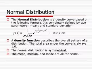
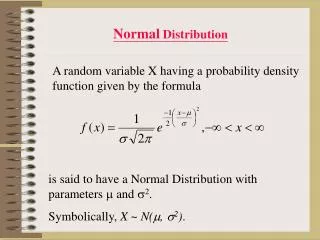
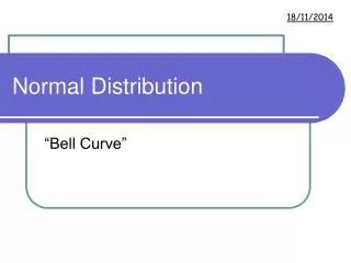
Normal distribution. Properties of the normal distribution. The center of the curve represents the mean (and median and mode). The curve is symmetrical around the mean. The tails meet the x-axis in infinity. The curve is bell-shaped. The area under the curve is 1 (by definition).

E N D
Properties of the normal distribution • The center of the curve represents the mean (and median and mode). • The curve is symmetrical around the mean. • The tails meet the x-axis in infinity. • The curve is bell-shaped. • The area under the curve is 1 (by definition).
Central Limit Theorem(Zentraler Grenzwertsatz) Der Mittelwert der Mittelwerte verschiedener Stichproben nähert sich dem wahren Mittelwert an. + Die Mittelwerte verschiedener Stichproben sind normalverteilt, selbst wenn das zu untersuchende Phänomen nicht normalverteilt ist.
Mean of the sample mean 4.75 + 3.0 + 3.0 + 2.75 + 2.5 = 3.2 5
The sample means are normally distributed (even if the phenomenon in the parent population is not normally distributed).
population sample
population one sample mean of this sample
population one sample mean of this sample distribution of many sample means
Are your data normally distributed? • The distribution in the parent population (normal, slightly skewed, heavily skewed). • The number of observations in the individual sample. • The total number of individual samples.
z scores x1 – x SD
Empirical rule 1.96
Parametric vs. non-parametrical tests • If you have ordinal data. • If you have interval data that is not normally distributed. • If you have interval data but cannot be certain if your data is normally distributed because you don’t have sufficient data (e.g. small number of samples, small individual samples). You use non-parametrical tests:
Confidence intervals Confidence intervals indicate a range within which the mean (or other parameters) of the true population lies given the values of your sample and assuming a certain probability. The standard error is the equivalent of the standard deviation for the sample distribution (i.e. the distribution based on the sample means).
Confidence intervals • The mean of the sample means. • The SDs of the sample means, i.e. the standard error. • The degree of confidence with which you want to state the estimation.
Standard error 0.292 5 - 1 = 0.2701
Confidence interval [degree of certainty] [standard error] = x [sample mean] +/–x = confidence interval
Confidence intervals 95% degree of certainty = 1.96 [z-score] Confindence interval of the first sample (mean = 1.5): 1.96 0.2701 = 0.53 1.5 +/- 0.53 = 0.97–2.03 We can be 95% certain that the population mean is located in the range between 0.97 and 2.03.
Exercise Mean: 7 SD: (2-7)2 + (5-7)2 + (6-7)2 + (7-7)2 + (10-7)2 + (12-7)2 6 -1 = 3.58 Standard error: 3.58 / 6 = 1.46 Confidence I.: 1.46 1.96 = 2.86 7 +/– 2.86 = 4.14 – 9.86