Sampling Distributions

1. Sampling Distributions

2. Sampling Distribution Introduction • In real life calculating parameters of populations is prohibitive because populations are very large. • Rather than investigating the whole population, we take a sample, calculate a statistic related to theparameter of interest, and make an inference. • The sampling distribution of the statistic is the tool that tells us how close is the statistic to the parameter.

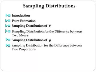
3. An estimatorof a population parameter is a sample statistic used to estimate or predict the population parameter. An estimateof a parameter is a particular numerical value of a sample statistic obtained through sampling. A point estimateis a single value used as an estimate of a population parameter. Sample Statistics as Estimators of Population Parameters A population parameteris a numerical measure of a summary characteristic of a population. A sample statisticis a numerical measure of a summary characteristic of a sample.

4. Estimators • The sample mean, , is the most common estimator of the population mean,  • The sample variance, s2, is the most common estimator of the population variance, 2. • The sample standard deviation, s, is the most common estimator of the population standard deviation, . • The sample proportion, , is the most common estimator of the population proportion, p.

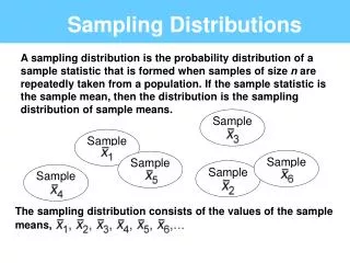
5. The sampling distribution of Xis the probability distribution of all possible values the random variable may assume when a sample of size n is taken from a specified population. Sampling Distribution of

6. x 1 2 3 4 5 6 p(x) 1/6 1/6 1/6 1/6 1/6 1/6 Sampling Distribution of the Mean • An example • A die is thrown infinitely many times. Let X represent the number of spots showing on any throw. • The probability distribution of X is E(X) = 1(1/6) + 2(1/6) + 3(1/6)+ ………………….= 3.5 V(X) = (1-3.5)2(1/6) + (2-3.5)2(1/6) + …………. …= 2.92

7. Throwing a dice twice – sampling distribution of sample mean • Suppose we want to estimate m from the mean of a sample of size n = 2. • What is the distribution of ?

8. Throwing a die twice – sample mean

9. 6/36 5/36 4/36 3/36 2/36 1/36 E( ) =1.0(1/36)+ 1.5(2/36)+….=3.5 V(X) = (1.0-3.5)2(1/36)+ (1.5-3.5)2(2/36)... = 1.46 1 1.5 2.0 2.5 3.0 3.5 4.0 4.5 5.0 5.5 6.0 The distribution of when n = 2

10. Sampling Distribution of the Mean 6

11. Notice that is smaller than sx. The larger the sample size the smaller . Therefore, tends to fall closer to m, as the sample size increases. Notice that is smaller than . The larger the sample size the smaller . Therefore, tends to fall closer to m, as the sample size increases. Sampling Distribution of the Mean

12. Relationships between Population Parameters and the Sampling Distribution of the Sample Mean The expected value of the sample meanis equal to the population mean: The variance of the sample meanis equal to the population variance divided by the sample size: The standard deviation of the sample mean, known as the standard error of the mean, is equal to the population standard deviation divided by the square root of the sample size:

13. n = 5 0 . 2 5 0 . 2 0 0 . 1 5 0 . 1 0 0 . 0 5 0 . 0 0 X n = 20 0 . 2 0 . 1 0 . 0 X Large n 0 . 4 0 . 3 0 . 2 0 . 1 0 . 0  - X The Central Limit Theorem When sampling from a population with mean  and finite standard deviation , the sampling distribution of the sample mean will tend to be a normal distribution with mean and standard deviationas the sample size becomes large (n >30). For “large enough” n: ) X ( P ) X ( P ) X ( f

14. Normal Uniform Skewed General Population n = 2 n = 30     X X X X The Central Limit Theorem Applies to Sampling Distributions from Any Population

15. The Central Limit Theorem (Example) Mercury makes a 2.4 liter V-6 engine, used in speedboats. The company’s engineers believe the engine delivers an average horsepower of 220 HP and that the standard deviation of power delivered is 15 HP. A potential buyer intends to sample 100 engines. What is the probability that the sample mean will be less than 217 HP?

16. The t is a family of bell-shaped and symmetric distributions, one for each number of degree of freedom. The expected value of t is 0. The variance of t is greater than 1, but approaches 1 as the number of degrees of freedom increases. The t distribution approaches a standard normal as the number of degrees of freedom increases. When the sample size is small (<30) we use t distribution. Standard normal t, df=20 t, df=10   Student’s t Distribution If the population standard deviation, , isunknown, replace with the sample standard deviation, s. If the population is normal, the resulting statistic: has a t distribution with (n - 1) degrees of freedom.

17. Sampling Distributions Finite Population Correction Factor If the sample size is more than 5% of the population size and the sampling is done without replacement, then a correction needs to be made to the standard error of the means.

18. Sampling Distribution of Standard Deviation of • is the finite correction factor. • is referred to as the standard error of the • mean. Finite Population Infinite Population • A finite population is treated as being • infinite if n/N< .05.

19. x = 32 m = 32.2 Sampling Distribution of the Sample Mean • The amount of soda pop in each bottle is normally distributed with a mean of 32.2 ounces and a standard deviation of 0.3 ounces. • Find the probability that a carton of four bottles will have a mean of more than 32 ounces of soda per bottle. • Solution • Define the random variable as the mean amount of soda per bottle. 0.9082

20. Sampling Distribution of the Sample Mean • Example • Dean’s claim: The average weekly income of M.B.A graduates one year after graduation is $600. • Suppose the distribution of weekly income has a standard deviation of $100. What is the probability that 25 randomly selected graduates have an average weekly income of less than $550? • Solution

21. n = 2 , p = 0 . 3 0 . 5 0 . 4 0 . 3 ) X ( P 0 . 2 0 . 1 0 . 0 0 1 2 X n=10,p=0.3 0 . 3 0 . 2 ) X ( P 0 . 1 0 . 0 0 1 2 3 4 5 6 7 8 9 1 0 X n = 1 5 , p = 0 . 3 0 . 2 ) X ( P 0 . 1 0 . 0 X 0 1 2 3 4 5 6 7 8 9 1 0 1 1 1 2 1 3 1 4 1 5 ^ p 7 15 10 15 15 15 0 15 1 15 2 15 3 15 4 15 5 15 6 15 8 15 9 15 11 15 12 15 13 15 14 15 The Sampling Distribution of the Sample Proportion, The sample proportionis the percentage of successes in n binomial trials. It is the number of successes, X, divided by the number of trials, n. Sample proportion: As the sample size, n, increases, the sampling distribution of approaches a normal distributionwith mean p and standard deviation

22. Normal approximation to the Binomial • Normal approximation to the binomial works best when • the number of experiments (sample size) is large, and • the probability of success, p, is close to 0.5. • For the approximation to provide good results two conditions should be met: np 5; n(1 - p) 5

23. Example • A state representative received 52% of the votes in the last election. • One year later the representative wanted to study his popularity. • If his popularity has not changed, what is the probability that more than half of a sample of 300 voters would vote for him?

24. Example • Solution • The number of respondents who prefer the representative is binomial with n = 300 and p = .52. Thus, np = 300(.52) = 156 andn(1-p) = 300(1-.52) = 144 (both greater than 5)