Download
1 / 54
550 likes | 830 Vues
Chapter 8 Binary Trees. Chapter 8 Binary Trees. 8.1 Trees, Binary Trees, and Binary Search Trees. Linked lists are linear structures and it is difficult to use them to organize a hierarchical representation of objects.

E N D
Chapter 8 Binary Trees 8.1 Trees, Binary Trees, and Binary Search Trees Linked lists are linear structures and it is difficult to use them to organize a hierarchical representation of objects. Although stacks and queues reflect some hierarchy, they are limited to only one dimension. To overcome this limitation, we create a new data type called a tree that consists of nodes and arcs. Unlike natural trees, these trees are depicted upside down with the root at the top and the leaves at the bottom.
Chapter 8 Binary Trees 8.1 Trees, Binary Trees, and Binary Search Trees The root is a node that has no parent; it can have only child nodes. Leaves, on the other hand, have no children. A tree can be defined recursively as the following: 1. Am empty structure is an empty tree 2. If t1, t2, …, tk are disjoint trees, then the structure whose root has its children the roots of t1, t2, …, tk is also a tree 3. Only structures generated by rules 1 and 2 are trees.
Chapter 8 Binary Trees 8.1 Trees, Binary Trees, and Binary Search Trees A path with length 3 Tree height= maximum level=4 Level=3+1=4 There is a unique path between any two nodes in a tree. (Hence a tree has no cycles.)
Chapter 8 Binary Trees 8.1 Trees, Binary Trees, and Binary Search Trees Examples: hierarchy of a university, genealogical tee, grammar tree, organic tree, … (Virtually all areas of science make use of trees to represent hierarchical structures.)
Chapter 8 Binary Trees 8.1 Trees, Binary Trees, and Binary Search Trees The definition of a tree does not impose any condition on the number of children of a given node. This number can vary from 0 to any integer. In hierarchical trees this is a welcome property. But, representing hierarchies is not the only reason for using trees. This chapter focuses on tree operations that allow us to accelerate the search process.
Chapter 8 Binary Trees 8.1 Trees, Binary Trees, and Binary Search Trees Consider a linked list of n elements. To locate an element, the search has to start from the beginning of the list and the list must be scanned until the element is found or the end of list is reached. (Best case: O(1), Worst case: O(n)) If all the elements are stored in an orderly tree, a tree where all elements are stored according to some predetermined criterion of ordering, the number of tests can be reduced substantially even when the element to be located is the one farthest away.
Chapter 8 Binary Trees 8.1 Trees, Binary Trees, and Binary Search Trees How to transform a list into a tree?
Chapter 8 Binary Trees 8.1 Trees, Binary Trees, and Binary Search Trees A binary tree is a tree whose nodes have at most two children (possibly empty) and each child is designated as either a left child or a right child. Examples:
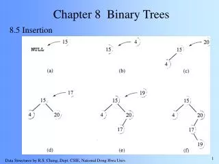
Chapter 8 Binary Trees 8.1 Trees, Binary Trees, and Binary Search Trees In a binary tree, if all nodes at all levels except the last had two children, then there would be 20 node at level 1 (root), 21 nodes at level 2, and generally, 2i nodes at level i+1. A tree satisfying this condition is referred to as a complete binary tree. In a complete binary tree, all non-terminal nodes have both their children, and all leaves are at the same level. Total number of nodes in a complete binary tree with level k is
Chapter 8 Binary Trees 8.1 Trees, Binary Trees, and Binary Search Trees A decision tree is a binary tree in which all nodes have either zero or two non-empty children. Example: sort a1, a2, a3 a1<a2 yes no a1<a3 a2<a3 yes yes no no a2<a3 a1<a3 a3<a1<a2 a3<a2<a1 yes yes no no a1<a2<a3 a1<a3<a2 a2<a1<a3 a2<a3<a1
Chapter 8 Binary Trees 8.1 Trees, Binary Trees, and Binary Search Trees Lemma: For all non-empty binary trees whose non-terminal nodes have exactly two non-empty children, the number of leaves m is greater than the number of non-terminal nodes k and m=k+1.
Chapter 8 Binary Trees 8.1 Trees, Binary Trees, and Binary Search Trees A binary search tree has the following property: if a node n of the tree contains the value v, then all values stored in its left subtree are less than v, and all values stored in the right subtree are greater than v. Examples of binary search trees
Chapter 8 Binary Trees 8.1 Trees, Binary Trees, and Binary Search Trees The corresponding binary search tree for the linked list Is it unique?
Chapter 8 Binary Trees 8.1 Trees, Binary Trees, and Binary Search Trees An algorithm for locating an element in the binary search tree is quite straightforward. For every node, compare the key to be located with the value stored in the node (starting from root, of course) currently pointed at. If the key is less than the value, go to the left subtree and try again. If it is greater than that value, try the right subtree. For example, to locate 31: To locate 28: Maximum number of searches the height of the tree found Not found
Chapter 8 Binary Trees 8.2 Implementing Binary Trees Array Representation Root However, it is hard to predict how many nodes will be created during a program execution. (Therefore, how many spaces should be reserved for the array?)
Chapter 8 Binary Trees 8.2 Implementing Binary Trees Dynamic linked structure struct node_rec { eltype key; struct node_rec *left, *right; }; typedef struct node_rec *tree_type; Key (data) left child right child
Chapter 8 Binary Trees 8.3 Searching a Binary Trees tree_type search1(tree_type node, eltype key) { while (node) if (key == node->key) return node; else if (key < node->key) node = =node->left; else node = node->right; return NULL; }
Chapter 8 Binary Trees 8.3 Searching a Binary Trees Using recursion: tree_type search2(tree_type node, eltype key) { if (node) if (key == node->key) return node; else if (key < node->key) return search2(node->left,key); else return search2(node->right,key); else return NULL; }
Chapter 8 Binary Trees 8.3 Searching a Binary Trees The complexity of searching is measured by the number of comparisons performed during the searching process. This number depends on the number of nodes encountered on the unique path leading from the root to the node being searched for. Therefore, the complexity is the length of the path leading to this node plus 1. It depends on the shape of the tree and the position of the node in the tree.
Chapter 8 Binary Trees 8.3 Searching a Binary Trees Search # of internal number comparisons path length 13 1 0 10 2 1 2 3 2 12 3 2 25 2 1 20 3 2 31 3 2 29 4 3 O(# of comparisons)=O(internal path length)
Chapter 8 Binary Trees 8.3 Searching a Binary Trees The (total) internal path length (IPL) is the sum of all path lengths of all nodes, which is calculated by summing (i-1)li over all levels i, where li is the number of nodes on level i. average (internal) path length=IPL/n In the worst case, when the tree turns into a linked list,
Chapter 8 Binary Trees 8.3 Searching a Binary Trees The best case occurs when all leaves in the tree of height h are in at most two levels and only nodes in the next to the last level can have one child. NO NO YES
Chapter 8 Binary Trees 8.3 Searching a Binary Trees IPL of best case < IPL of complete binary tree with the same height Therefore, we approximate the average path length for best case tree by the average path length of a complete binary tree of the same height, h. For a complete binary tree of height h, IPL=
Chapter 8 Binary Trees 8.3 Searching a Binary Trees The total number of nodes in a complete binary tree with height h is n=2h-1. Therefore, O(pathbest)=O(logn) The average case is somewhere between (n-1)/2 and log(n+1)-2. Is a search for a node in an average position in a tree closer to O(n) or O(logn)? First, the average shape of the tree has to be represented computationally.
Chapter 8 Binary Trees 8.3 Searching a Binary Trees Assume that the tree contains nodes 1 through n. If i is the root, then its left subtree has i-1 nodes, and its right subtree has n-i nodes. If pathi-1 and pathn-i are average paths in these subtrees, then the average path of this tree is n-i nodes i-1 nodes
Chapter 8 Binary Trees 8.3 Searching a Binary Trees The left subtree can have any number of nodes {from 1(i=1) to n-1 (i=n)}. Therefore, the average path length of an average tree is obtained by averaging all values of pathn(i) over all values of i. This gives this formula
Chapter 8 Binary Trees 8.4 Tree Traversal Tree traversal is the process of visiting each node in the tree exactly one time. (It does not specify the order in which the nodes are visited.) Therefore, 8!=40320 possible traversals for the example tree. Only a few of them have regularity and are useful.
Chapter 8 Binary Trees 8.4.1 Breadth-First Traversal Breadth-first traversal is visiting each node starting from the root and moving down level be level, visiting nodes on each level from left to right. Breadth-first traversal sequence: 13, 10, 25, 2, 12, 20, 31, 29
Chapter 8 Binary Trees 8.4.1 Breadth-First Traversal Implementation of breadth-first traversal is quite straightforward when a queue is used. After a node is visited, its children, if any, are placed at the end of the queue, and the node at the beginning of the queue is visited. Considering that for a node on level n, its children are on level n+1, by placing these children at the end of the queue, they are visited after all nodes from level n are visited. Level n+1 nodes
Chapter 8 Binary Trees 8.4.1 Breadth-First Traversal void breadth_first(tree_type node) { if (node) { enq(node,queue); while (!empty(queue)) { node=deq(queue); visit(node); if (node->left) enq(node->left,queue); if (node->right) enq(node->right,queue); } } }
Chapter 8 Binary Trees 8.4.2 Depth-First Traversal Depth-first traversal proceeds as far as possible to the left (or right), then backs up until the first crossroad, goes one step to the right (or left), and again as far as possible to the left (or right). Repeat this process until all nodes are visited.
Chapter 8 Binary Trees 8.4.2 Depth-First Traversal There are three tasks of interest in this type of traversal: V: visiting a node L: traversal the left subtree R: traversal the right subtree An orderly traversal takes place if these tasks are performed in the same order for each node. So there are six possible traversals: VLR, VRL, LVR, RVL, LRV, RLV. VLR: 13,10,2,12,25,20,31,29 VRL: 13 25,31,29,20,10,12,2 LVR: 2,10,12,13,20,25,29,31 RVL: 31,29,25,20,13,12,10,2 LRV: 2,12,10,20,29,31,25,13 RLV: 29,31,20,25,12,2,10,13
Chapter 8 Binary Trees 8.4.2 Depth-First Traversal Assume the move is always from left to right, then there are three standard traversals: VLR: preorder (binary) tree traversal LVR: inorder tree traversal LRV: postorder tree traversal Preorder(tree_type node) { if (node) { visit(node); preorder(node->left); preorder(node->right); } } inorder(tree_type node) { if (node) { inorder(node->left); visit(node); inorder(node->right); } } Postorder(tree_type node) { if (node) { postorder(node->left); preorder(node->right); visit(node); } }
Chapter 8 Binary Trees 8.4.2 Depth-First Traversal Non-recursive version Void iterative_preorder(tree_type p) { if (p) { push(p,stack); while(!empty(stack)) { p=pop(stack); visit(p); if (p->right) push(p->right,stack); /*left child pushed */ if(p->left) push(p->left,stack); /* after right to be */ } /* at the top of the */ } /* stack */ }
Chapter 8 Binary Trees 8.4.2 Depth-First Traversal Non-recursive version Can we so easily transform the non-recursive version of preorder traversal into a non-recursive postorder traversal? Will moving visit() to be after both push() do? Unfortunately not. What matters here is that visit() has to follow pop() and the latter has to precede both calls of push(). Therefore, non-recursive implementations of inorder and postorder traversals have to be developed independently.
Chapter 8 Binary Trees 8.4.2 Depth-First Traversal Non-recursive version A non-recursive version of postorder traversal can be obtained rather easily if we observe that the sequence generated by a left-to-right postorder traversal (a LRV order) is the same as the reversed sequence generated by a right-to-left preorder traversal (a VRL order). VLR: 13,10,2,12,25,20,31,29 VRL: 13 25,31,29,20,10,12,2 LVR: 2,10,12,13,20,25,29,31 RVL: 31,29,25,20,13,12,10,2 LRV: 2,12,10,20,29,31,25,13 RLV: 29,31,20,25,12,2,10,13
Chapter 8 Binary Trees 8.4.2 Depth-First Traversal Non-recursive version Void iterative_postorder(tree_type p) { if (p) { push(p,stack1); while(!empty(stack1)) { p=pop(stack1); push(p,stack2); if (p->left) push(p->left,stack1); /*right child pushed */ if(p->right) push(p->right,stack1); /* after left to be */ } /* at the top of the */ } /* stack (VRL order) */ while(!empty(stack2)) { p=pop(stack2); visit(p); } } Reverse the sequence using another stack
Chapter 8 Binary Trees 8.4.2 Depth-First Traversal Non-recursive version Only the root are stacked. Void iterative_inorder(tree_type p) { while (p) { while (p) { if (p->right) push(p->right,stack); push(p,stack); p=p->left; } p=pop(stack); while (!empty(stack) && !(p->right)) { visit(p); p=pop(stack); } visit(p); if (!empty(stack)) p=pop(stack); else p=NULL; } } Stack the right child (if any) and the node itself when going to the left. Pop a node with no left child. Visit it and all nodes with no right child. Visit the node with a right child and repeat the procedure for the right subtree.
Chapter 8 Binary Trees 8.4.3 Stackless Depth-First Traversal Threaded Trees Either recursive or non-recursive traversal procedures uses a stack to store information about nodes. The concern is that some additional time has to be spent to maintain the stack, and some more space has to be set aside for the stack itself. In the worst case, when the tree is unfavorably skewed, the stack may hold information about almost every node of the tree, a serious concern for very large trees. Question: What is the worst case tree for preorder, inorder, or postorder?
Chapter 8 Binary Trees 8.4.3 Stackless Depth-First Traversal Threaded Trees It would be more efficient to incorporate the stack as part of the tree. This is done by incorporating threads in a given node. Threads are pointers to the predecessor and successor of the node according to a certain sequence, and trees whose nodes use threads are called threaded trees. Four pointer fields (two for children, two for predecessor and successor) would be needed for each node in the tree, which again takes up valuable space.
Chapter 8 Binary Trees 8.4.3 Stackless Depth-First Traversal Threaded Trees The problem can be solved by overloading existing pointer fields. An operator is called overloaded if it can have different meanings; the * operator in C is a good example, since it can be used as the multiplication operator or for dereferencing pointers. In trees, left or right pointers are pointers to children, but they can also be used as pointers to predecessors and successors, thereby overloaded with meaning.
Chapter 8 Binary Trees 8.4.3 Stackless Depth-First Traversal Threaded Trees For an overloaded operator, context is always a disambiguating factor. In trees, however, a new field has to be used to indicate the current meaning of the pointers. The left pointer is either a pointer to the left child or to the predecessor. Analogously, the right pointer will point either to the right subtree or to the successor. The meaning of predecessor and successor differs depending on the sequence under scrutiny.
Chapter 8 Binary Trees 8.4.3 Stackless Depth-First Traversal Threaded Trees
Chapter 8 Binary Trees 8.4.3 Stackless Depth-First Traversal Threaded Trees Figure 8.13 suggests that both pointers to predecessors and to successors have to be maintained, which is not always the case. It may be sufficient to use only one thread as shown in the following implementation of the inorder traversal of a threaded tree, which requires only pointers to successors.
Chapter 8 Binary Trees 8.4.3 Stackless Depth-First Traversal Void threaded_inorder(threaded_tree_type p) { threaded_tree_type prev; if (p) { /* process only ono-empty trees */ while (p->left) p=p->left; /* go to the leftmost node */ while (p) { visit(p); prev=p; p=p->right; /* go to the right node */ if (p && prev->successor ==0) /* If the right pointer */ while (p->left) p=p->left; /* is not a successor */ } /* pointer, go to the */ } /* leftmost node */ }
Chapter 8 Binary Trees 8.4.3 Stackless Depth-First Traversal Only an extra bit is needed in tree structure. Struct node_rec { eltype key; unsigned successor:1; struct node_rec *left, *right; } typedef struct node_rec *threaded_tree_type;
Chapter 8 Binary Trees 8.4.3 Stackless Depth-First Traversal Traversal through Tree Transformation It is possible to traverse a tree without using any stack or threads. There are many such algorithms, all of them made possible by making temporary changes in the tree during traversal. These changes consist of reassigning new values to some pointer fields. However, the tree may temporarily lose its tree structure which needs to be restored before traversal is finished.
Chapter 8 Binary Trees 8.4.3 Stackless Depth-First Traversal Traversal through Tree Transformation First, it is easy to notice that inorder traversal is very simple for degenerate trees, in which no node has a left child. Therefore, the usual three steps, LVR, turn into two steps, VR. No information needs to be retained about the current status of the node being processed before traversing its left child, simply because there is no left child. Morris’ algorithm takes into account this observation by temporarily transforming the tree so that the node being processed has no left child; hence, this node can be visited and its right subtree processed.
Chapter 8 Binary Trees 8.4.3 Stackless Depth-First Traversal Traversal through Tree Transformation while not finished /* for inorder traversal */ if node has no left descendant visit it; go to the right; else make this node right child of the rightmost node in its left descendent; go to this left descendant; Inorder: LVR should be after in inorder. the rightmost node