Chapter 8 Binary Trees

1. Chapter 8 Binary Trees 8.5 Insertion

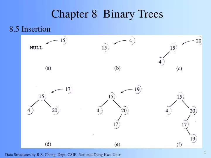
2. Chapter 8 Binary Trees 8.5 Insertion Void insert(tree_type *root_addr, eltype key) { tree_type p, previous=NULL, new_node, malloc(); new_node=malloc(sizeof(struct node_rec)); new_node->left=new-node->right=NULL; new_node->key=key; p=*root_addr; while (p) { previous=p; if (p->key > key) p=p->left; else p=p->right; } if (!*root_addr) *root_addr = new_node; else if (previous->key > key) previous->left=new_node; else previous->right=new_node; }

3. Chapter 8 Binary Trees 8.5 Insertion The procedure is not sufficiently flexible because the assignment statement and the comparison is not general enough. It can handle only numbers. To generalize the assignment and the comparisons, we use pointers to functions and pass both a pointer to an assignment function and a pointer to a comparison function as parameters to the procedure. void insert2( tree_type *root_addr, eltype *key, int (*comparison) (eltype *, eltype *), void (*copy)(eltype *,eltype *))

4. Chapter 8 Binary Trees 8.5 Insertion Inserting nodes into a threaded tree (for inorder traversal)

5. Chapter 8 Binary Trees 8.6 Deletion What if the node to be deleted has two children? In this case, no one-step operation can be performed since the parent’s right or left pointer cannot point to both children at the same time.

6. Chapter 8 Binary Trees 8.6 Deletion 8.6.1 First Solution Symmetrically, the node with the lowest value can be found in the right subtree and made a parent of the left subtree.

7. Chapter 8 Binary Trees 8.6 Deletion 8.6.1 First Solution Void delete_by_merging (tree_type *node) { tree_type tmp=*node; if (*node) { if (!(*node)->right) /* the node has no right child, its left */ *node=(*node)->left /* child it attached to parent */ else if (!(*node)->left) *node=(*node)->right; else { tmp=(*node)->left; /* move left and then right as far */ while (tmp->right) /* as possible */ tmp=tmp->right; tmp->right=(*node)->right; /* establish the link between the */ tmp=*node; /* rightmost node of the left subtree */ *node=(*node)->left; /* and the right subtree */ } free(tmp); }}

8. Chapter 8 Binary Trees 8.6 Deletion 8.6.1 First Solution

9. Chapter 8 Binary Trees 8.6 Deletion 8.6.1 First Solution Tree height increased

10. Chapter 8 Binary Trees 8.6 Deletion 8.6.1 First Solution Tree height decreased

11. Chapter 8 Binary Trees 8.6 Deletion 8.6.2 Second Solution Delete by copying

12. Chapter 8 Binary Trees 8.6 Deletion 8.6.2 Second Solution Delete by copying

13. Chapter 8 Binary Trees 8.6 Deletion 8.6.2 Second Solution Void delete_by_copying (tree_type *node) { tree_type previous, tmp=*node; if (*node) { if (!(*node)->right) /* the node has no right child, its left */ *node=(*node)->left /* child it attached to parent */ else if (!(*node)->left) *node=(*node)->right; else { tmp=(*node)->left; /* move left and then right as far */ previous=*node; while (tmp->right) { /* as possible */ previous=tmp; tmp=tmp->right; } (*node)->key=tmp->key; /* copy key data */ if (previous == * node) previous->left=tmp->left; else previous->right=tmp->left; } free(tmp); }} No right subtree

14. Chapter 8 Binary Trees 8.7 Balancing a Tree balancing

15. Chapter 8 Binary Trees 8.7 Balancing a Tree A binary tree is height-balanced or simply balanced if the difference in height of both subtrees of any node is either zero or one. Also, a tree is considered perfectly balanced if it it balanced and all leaves are to be found on one level or two levels. Balanced but not perfectly

16. Chapter 8 Binary Trees 8.7 Balancing a Tree What is the benefit of balancing a binary tree? For example, if 10,000 elements are stored in a perfectly balanced tree, then the tree is of height In practical terms, this means that if 10,000 elements are stored in a perfectly balanced tree, then at most fourteen nodes have to be checked to locate a particular element. This is a substantial difference compared to the 10,000 tests needed in a linked list.

17. Chapter 8 Binary Trees 8.7 Balancing a Tree There are a number of techniques to properly balance a binary tree. 1. Some of them consist of constantly restructuring the tree when elements arrive and lead to an unbalanced tree. 2. Some of them consist of reordering the data themselves and then building a tree, if an ordering of the data guarantees that the resulting tree will be balanced.

18. Chapter 8 Binary Trees 8.7 Balancing a Tree First step: sort the input data

19. Chapter 8 Binary Trees 8.7 Balancing a Tree Void balance(int data[], int first, int last) { int middle=first+(last-first)/2; insert(&root, data[middle]); balance(data,first,middle-1); balance(data,middle+1,last); } This algorithm has one serious drawback: all data must be put in an array before the tree can be created. But the data can be transferred from an unbalanced tree to the array using inorder traversal. The tree can now be deleted and recreated using balance().

20. Chapter 8 Binary Trees 8.7 Balancing a Tree 8.7.1 The DSW Algorithm The building block for tree transformations in DSW algorithm is the rotation. The right rotation of the node Ch about its parent Par is performed according to the following algorithm: RotateRight(Gr,Par,Ch) if Par is not the root of the tree /* i.e., if GR is not NULL */ Gr becomes Ch’s parent by replacing Par; right subtree of Ch becomes left subtree of Par; Ch acquires Par as its right child;

21. Chapter 8 Binary Trees 8.7 Balancing a Tree 8.7.1 The DSW Algorithm Left rotation of Par about Ch Right rotation of Ch about Par

22. Chapter 8 Binary Trees 8.7 Balancing a Tree 8.7.1 The DSW Algorithm Basically, the DSW algorithm transforms an arbitrary binary search tree into a linked list-like tree, called a backbone or vine, and then this elongated tree is transformed in a series of passes into a perfectly balanced tree by repeatedly rotating every second node of the backbone about its parent. CreateBackbone(root,n) tmp=root; while (tmp!= NULL) if tmp has a left child rotate this child about tmp; set tmp to the child which just became parent; else set tmp to its right child;

23. Chapter 8 Binary Trees 8.7 Balancing a Tree 8.7.1 The DSW Algorithm Transforming a binary search tree into a backbone

24. Chapter 8 Binary Trees 8.7 Balancing a Tree 8.7.1 The DSW Algorithm In the worst case, the while loop would be executed 2n-1 times with n-1 rotations performed where n is the number of nodes in the tree; the run time of the first phase is O(n). When will this worst case occur? In the second phase, in each pass down the backbone, every second node is (reverse right) rotated about its parent. The first pass is used to account for the difference between the number n of nodes in the current tree and the number of nodes in the closest complete binary tree.

25. Chapter 8 Binary Trees 8.7 Balancing a Tree 8.7.1 The DSW Algorithm CreatePerfectTree(n) make n-m rotations starting from the top of the backbone; while (m>1) m=m/2; make m rotations starting from the top of the backbone;

26. Chapter 8 Binary Trees 8.7 Balancing a Tree 8.7.1 The DSW Algorithm 3/2=1 rotations 7/2=3 rotations n-m=9-7=2 rotations 7=23-1, nodes for a complete binary tree

27. Chapter 8 Binary Trees 8.7 Balancing a Tree 8.7.1 The DSW Algorithm To compute the complexity of the tree building phase, observe that The number of rotations can be given now by the formula That is, the number of rotations is O(n). Because creating a backbone also requires at most O(n) rotations, the cost of DSW algorithm is O(n), optimal in terms of time and space, since it grows linearly with n.

28. Chapter 8 Binary Trees 8.7 Balancing a Tree 8.7.2 AVL Trees Tree rebalancing can be performed locally if only a portion of the tree is affected when changes are required after an element is inserted into or deleted from the tree. An AVL tree (originally called an admissible tree) is a tree in which the height of left and right subtrees of every node differ by at most one.

29. Chapter 8 Binary Trees 8.7 Balancing a Tree 8.7.2 AVL Trees Balance factor= (H of right tree)- (H of left tree) For an AVL tree, all balance factors should be +1, 0, or -1.

30. Chapter 8 Binary Trees 8.7 Balancing a Tree 8.7.2 AVL Trees Notice that the definition of the AVL tree is the same as the definition of the balanced tree. However, the concept of the AVL tree always implicitly includes the techniques for balancing the tree. Moreover, the technique for balancing AVL trees does not guarantee that the resulting tree is perfectly balanced. The definition of an AVL tree indicates that the minimum number of nodes in a tree is determined by the recurrence relation AVLh=AVLh-1+AVLh-2+1 where AVL0=0 and AVL1=1 are the initial conditions. Numbers generated by this recurrence formula are called Leonardo numbers.)

31. Chapter 8 Binary Trees 8.7 Balancing a Tree 8.7.2 AVL Trees The formula leads to the following bounds on the height h of an AVL tree depending on the number of nodes n: Therefore, h is bounded by O(logn); the worst case search requires O(logn) comparisons. If the balance factor of any node in an AVL tree becomes less than -1 or greater than 1, the tree has to be balanced. An AVL tree can become out of balance in four situations, but only two of them need to be analyzed; the remaining two are symmetrical.

32. Chapter 8 Binary Trees 8.7 Balancing a Tree 8.7.2 AVL Trees The first case: inserting a node in the right subtree of the right child Left rotation

33. Chapter 8 Binary Trees 8.7 Balancing a Tree 8.7.2 AVL Trees The second case: inserting a node in the left subtree of the right child In more detail insert

34. Chapter 8 Binary Trees 8.7 Balancing a Tree 8.7.2 AVL Trees The second case: inserting a node in the left subtree of the right child Right rotation Left rotation

35. Chapter 8 Binary Trees 8.7 Balancing a Tree 8.7.2 AVL Trees In these two cases, the tree P is considered as a stand-alone tree. However, P can be part of a larger AVL tree. If a tree is inserted into the tree and the balance of P is disturbed and then restored, does extra work need to be done to the predecessors of P? Fortunately not. Note that the heights of the trees resulting from the rotations are the same as the heights of the tree before insertion. The only problem is to find a node P (the lowest ancestor node) for which the balance factor becomes unacceptable after a node has been inserted.

36. Chapter 8 Binary Trees 8.7 Balancing a Tree 8.7.2 AVL Trees This node can be detected by moving up toward the root from the position in which the new node has been inserted and by updating the balance factors of the node encountered. If a node with a 1 balance factor is encountered, the balanced factor may be changed to 2 and the root of the subtree to be balanced is found. However, if the balance factors on the path are all zero, the balance factors may be changed to 1, but no rotations would be needed.

37. Chapter 8 Binary Trees 8.7 Balancing a Tree 8.7.2 AVL Trees A new node is inserted, but no height adjustments are needed.

38. Chapter 8 Binary Trees 8.7 Balancing a Tree 8.7.2 AVL Trees One rotation is required to restore the height balance.

39. Chapter 8 Binary Trees 8.7 Balancing a Tree 8.7.2 AVL Trees Deletion may be more time-consuming that insertion. First, we apply delete_by_copying() to delete a node. After a node has been deleted, updating balance factors is performed from the parent of the deleted node up to the node. For each node in this path, whose balance factor becomes 2, a single or double rotation has to be performed to restored the balance of the subtree. Importantly, the rebalancing does not stop after the first unbalanced node. This means that deletion may lead to at most O(logn) rotations.

40. Chapter 8 Binary Trees 8.7 Balancing a Tree 8.7.2 AVL Trees Three cases of left deletion (The other symmetrical cases are right deletion resulting in P=-2): Case 1:

41. Chapter 8 Binary Trees 8.7 Balancing a Tree 8.7.2 AVL Trees Three cases of left deletion: Case 2:

42. P Chapter 8 Binary Trees +2 R +1 8.7 Balancing a Tree Q +1 h-1 8.7.2 AVL Trees h-1 Three cases of left deletion: h-2 h-1 Case 3: Two other subcases for R=0 and R=+1

43. Chapter 8 Binary Trees 8.8 Self-Adjusting Trees Is balancing always necessary or a good strategy when inserting a new element? AVL: restructuring the tree locally DSW algorithm: recreating the tree Performance can be improved by balancing the tree, but this is not the only method which can be used. Another approach begins with the observation that not all elements are used with the same frequency. The more frequent a node is accessed, the closer it should be to the root.

44. Chapter 8 Binary Trees 8.8 Self-Adjusting Trees Therefore, the strategy in self-adjusting trees is to restructure trees only by moving up the tree those elements which are used more often, creating a kind of “priority tree.” The frequency of accessing nodes can be determined in a variety of ways. Each node can have a counter field which records the number of times the element has been used for any operation. (Information may be obsolete. That is, it may be the most frequently accessed node in a long time ago.)

45. Chapter 8 Binary Trees 8.8 Self-Adjusting Trees In a less sophisticated approach, it is assumed that an element being accessed has a good chance of being accessed again soon. Therefore, it is moved up the tree. No restructuring is performed for new elements. This assumption may lead to promoting elements which are occasionally accessed, but the overall tendency is to move up elements with a high frequency of access, and for the most part, these elements will populate the first few levels of the tree.

46. Chapter 8 Binary Trees 8.8 Self-Adjusting Trees 8.8.1 Self-Restructuring Trees

47. Chapter 8 Binary Trees 8.8 Self-Adjusting Trees 8.8.1 Self-Restructuring Trees Using the single rotation strategy, frequently accessed elements will eventually be moved up close to the root. In the move-to-the-root strategy, it is assumed that the elements being accessed has a high probability to be accessed again. These strategies, however, do not work very well in unfavorable situations, when the binary tree resembles a linked list rather than a tree. In this case, the shape of the tree is only slowly improved.

48. Chapter 8 Binary Trees 8.8 Self-Adjusting Trees 8.8.1 Self-Restructuring Trees Moving T to the root

49. Chapter 8 Binary Trees 8.8 Self-Adjusting Trees 8.8.1 Self-Restructuring Trees Moving S to the root

50. Chapter 8 Binary Trees 8.8 Self-Adjusting Trees 8.8.2 Splaying A modification of the moving-to-the-root strategy is called splaying, which applies single rotations in pairs in an order depending on the links between the child, parent, and grandparent. R: the node accessed, Q: the parent, P: the grandparent case 1: node R’s parent is the root case 2: homogeneous configuration: node R is the left child of Q and Q is the left child of P (or R and Q are both right child) case 3: heterogeneous configuration: node R is the right child of Q and Q is the left child of P (or R is the left child of Q and Q is the right child of P)