Continuous Probability Distributions
430 likes | 1.04k Vues
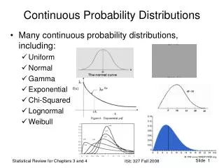
Continuous Probability Distributions. Week 6 GT00303. CONTINUOUS RANDOM VARIABLE A random variable that takes on an infinite number of values within a given range. It is usually the result of some type of measurement. EXAMPLES The length of each song on the latest Tim McGraw album.

Continuous Probability Distributions
E N D
Presentation Transcript
Continuous Probability Distributions Week 6 GT00303
CONTINUOUS RANDOM VARIABLE A random variable that takes on an infinite number of values within a given range. It is usually the result of some type of measurement. EXAMPLES The length of each song on the latest Tim McGraw album. The weight of each student in this class. The temperature outside as you are reading this book. The amount of money earned by each of the more than 750 players currently on Major League Baseball team rosters. 6-2
We cannot list the possible values because there is an infinite number of them. Since there is an infinite number of values, the probability of each individual value is virtually ZERO. E.g. P(X=2) = 0, P(X=5) = 0 Hence, in a continuous setting, point probabilities are ZERO. It is more meaningful to determine the probability of a range of values. E.g. P(X ≤ 2) or P(2 ≤ X ≤ 5). 6-3
Probability Density Function (PDF) A function f(x) is called a probability density function (over the range a ≤ X ≤ b if it meets the following requirements: • f(x) ≥ 0 for all between a and b, and • The total area under the curve between a and b is 1.0. f(x) area=1 a b x 6-4
Uniform Distribution The uniform probability distribution is perhaps the simplest distribution for a continuous random variable. f(x) area=1 a b x For PDF, the total area under the curve (line) is 1. So, how much the height should be? 6-5
Mean of the Uniform Distribution SD of the Uniform Distribution 6-6
Illustration 1: The amount of gasoline sold daily at a service station is uniformly distributed with a minimum of 2,000 gallons and a maximum of 5,000 gallons. Find the probability that daily sales will fall between 2,500 and 3,000 gallons. P(2500 ≤ X ≤ 3000) f(x) 2,000 5,000 x 6-7
There is about 16.67% chance that between 2500 and 3000 gallons of gas will be sold on a given day. What is the probability that the service station will sell at least 4000 gallons? P(X ≥ 4000) f(x) 2,000 5,000 x 6-8
What is the probability that the service station will sell exactly 2500 gallons? P(X = 2500) f(x) 2,000 5,000 x Hence, in a continuous setting, point probabilities are ZERO. 6-9
Illustration 2: Southwest Arizona State University provides bus service to students while they are on campus. A bus arrives at the North Main Street and College Drive stop every 30 minutes between 6 A.M. and 11 P.M. during weekdays. Students arrive at the bus stop at random times. The time that a student waits is uniformly distributed from 0 to 30 minutes. How long will a student “typically” have to wait for a bus? 6-10
What is the standard deviation of the waiting time? What is the probability a student will wait more than 25 minutes? 6-11
What is the probability a student will wait between 10 and 20 minutes? 6-12
Normal Distribution The normal distribution is the most important of all probability distributions. The normal distribution is bell shaped and symmetrical about the mean 6-13
The PDF of a normal distribution is given by: The normal distribution is fully defined by two parameters: its standard deviation andmean Unlike the range of the uniform distribution (a ≤ x ≤ b), normal distributions range from minus infinity to plus infinity 6-14
The normal distribution is described by two parameters: μ and σ. Increasing the mean shifts the normal curve to the right. 6-15
The normal distribution is described by two parameters: μ and σ. Increasing the standard deviation flattens the normal curve. 6-16
0 1 1 Standard Normal Distribution A normal distribution whose mean is zero and standard deviation is one is called the standard normal distribution. Any normal distribution can be converted to a standard normal distribution with simple algebra. This makes statistical inferences much easier. 6-17
We can convert any normal random variable to a standard normal random variable (Z variable) as follows: This shifts the mean of X to zero 0 Some advice: always draw a picture! This changes the shape of the curve 6-18
Area under the Normal Curve The total area under the normal curve is 1.00; half of the the area (0.5) under the normal curve is to the right of μ, and the other half (0.5) to the left of μ. 6-19
Illustration 3: Suppose that at another gas station the daily demand for regular gasoline is normally distributed with a mean of 1,000 gallons and a standard deviation of 100 gallons. The station manager has just opened the station for business and notes that there is exactly 1,100 gallons of regular gasoline in storage. The next delivery is scheduled later today at the close of business. The manager would like to know the probability that he will have enough regular gasoline to satisfy today’s demands. X = Daily demand for regular gasoline (in gallons) P(X < 1100) = ?? 6-20
P(X < 1100) Convert X into standard normal random variable (Z). +1 +2 -1 -3 +3 -2 Use Standard Normal Probability Table! 6-21
P(Z < 1) = 0.8413 6-22
Standard Normal Table The standard normal table provides P(Z < z), that is the total area to the left of z. For standard normal table, we can’t find the probability that Z is equal to a specific value of z, say P(Z = 1.2). This is because normal random variable is continuous and the probability that a continuous random variable is equal to any single value is ZERO (Point probabilities are ZERO). 6-23
P(Z < -1.52) = 0.0643 P(Z > 1.8) = 1 – P(Z < 1.8) = 1 – 0.9641 = 0.0359 6-24
P(-1.3 < Z < 2.1) = P(Z < 2.1) – P(Z < -1.3) = 0.9821 – 0.0968 = 0.8853 Can you get: P(-2.10 < Z < 0) = 0.4821 P(0 < Z < 2.5) = 0.4938 6-25
Illustration 4: Consider an investment whose return is normally distributed with a mean of 10% and a standard deviation of 5%. • Determine the probability of losing money. • Find the probability of losing money when the standard deviation is equal to 10%. X = Return for an investment (in %) 6-26
Determine the probability of losing money. P(X < 0) = ?? P(Z < -2) = 0.0228 • Find the probability of losing money when the standard deviation is equal to 10%. P(X < 0) = ?? P(Z < -2) = 0.1587 6-27
Finding Value of z Given an area (A) under the curve, what is the corresponding value of z (zA) on the horizontal axis that gives us this area? • This is particularly useful when performing hypothesis testing! 6-28
Illustration 5: In hypothesis testing, an important step is to find the critical value. Suppose that this is a one-tail test and the level of significance is 10%. What is the critical value of z? P(Z < z) = 0.90 z = 1.28 6-29
Illustration 6: The lifetimes of the heating element in a Heatfast electric oven are normally distributed, with a mean of 7.8 years and a standard deviation of 2.0 years. If the element is guaranteed for 2 years, what is the probability that the ovens sold will need replacement in the guarantee period because of element failure? Heatfast is reconsidering the length of the guarantee period on heating elements. Calculate the length of guarantee period such that Heatfast would expect to replace a maximum of 1% of sets due to element failure. 6-30
X = Lifetime of a heating element (in years) What is the probability that the ovens sold will need replacement in the guarantee period? P(X < 2) = ?? P(Z < -2.9) = 0.0019 @ 0.19% 6-31
Calculate the length of guarantee period such that Heatfast would expect to replace a maximum of 1% of sets due to element failure. P(Z < z) = 0.01 0.0019 z = -2.33 What is the corresponding X value? X=2 0.01 z = ??? X = ??? 6-32
Exponential Distribution The exponential distribution has this probability density function: The exponential distribution usually describes inter-arrival situations such as: • The service times in a system. • The time between “hits” on a web site. • The lifetime of an electrical component. • The time until the next phone call arrives in a customer service center Characteristics: 1. Positively skewed, similar to the Poisson distribution (for discrete variables). 2. Described by only one parameter, which we identify as λ, often referred to as the “rate” of occurrence parameter. 3. As λ decreases, the shape of the distribution becomes “less skewed.” 6-33
Illustration 7: The lifetime of an alkaline battery (measured in hours) is exponentially distributed with λ = 0.05 Find the probability a battery will last between 10 & 15 hours. 6-34
P(10<X<15) There is about 13.41% chance a battery will only last 10 to 15 hours 6-35
Other Continuous Distributions Student t Distribution The degrees of freedom () defines the Student t distribution. As the number of degrees of freedom increases, the t distribution approaches the standard normal distribution 6-36
The degrees of freedom () defines the 2 distribution. Chi-Squared (2) Distribution The 2 distribution starts at zero (is non-negative) and is not symmetrical. 6-37
F Distribution The degrees of freedom () defines the F distribution. The Fdistribution starts at zero (is non-negative) and is not symmetrical. 6-38