Download

1 / 51
550 likes | 974 Vues
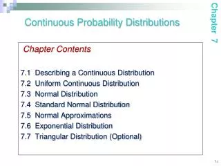
Continuous Probability Distributions. Chapter 7. Modified by Boris Velikson, fall 2009. GOALS. Understand the difference between discrete and continuous distributions. Compute the mean and the standard deviation for a uniform distribution.

E N D
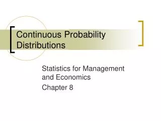
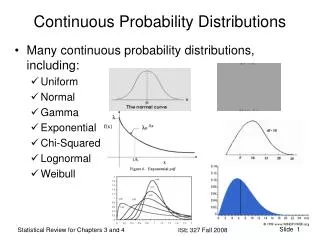
Continuous Probability Distributions Chapter 7 Modified by Boris Velikson, fall 2009
GOALS • Understand the difference between discrete and continuous distributions. • Compute the mean and the standard deviation for a uniform distribution. • Compute probabilities by using the uniform distribution. • List the characteristics of the normal probability distribution. • Define and calculate z values. • Determine the probability an observation is between two points on a normal probability distribution. • Determine the probability an observation is above (or below) a point on a normal probability distribution. • Use the normal probability distribution to approximate the binomial distribution.
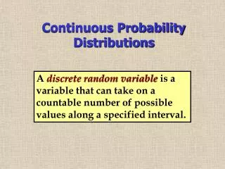
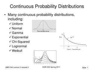
The Uniform Distribution A Discretedistribution is based on random variables which can assume only clearly separated values A Continuous distribution usually results from measuring something. Discrete distributions studied include: Binomial Hypergeometric (no, we did not) Poisson. Continuous distributions include: Uniform Normal Others
The Uniform Distribution The uniform probability distribution is perhaps the simplest distribution for a continuous random variable. • Suppose the time to access the McGraw-Hill web page is uniformly distributed with a minimum time of 20 ms and a maximum time of 60 ms. Then • The probability that 20 ms t 60 ms is 1 • The probability that 20 ms t 40 ms is 0.5 • The probability that 40 ms t 60 ms is 0.5 • The probability that 30 ms t 40 ms is 0.25 etc. • The probability is proportional to the length of the interval within the total interval.
P 1/(b-a) t 0 a c d b The Uniform Distribution • For continuous distributions, we represent probabilities by areas on the graph. The total area is 1, therefore the height of the rectangle is 1/(b – a), if we assume that a t b. • The probability that t belongs to a shorter interval [c,d] is then (d-c)/(b-a). (We assume that both c and dlie between a and b.)
P 1/(b-a)=1/40 t, ms 0 20 30 40 50 60 P 1/(b-a)=1/40 t, ms 40 0 20 30 50 60 The Uniform Distribution • The probability that t belongs to the interval [40,50] is the same as for [30,40]or for any other interval of length 10. It equals (d-c)/(b-a)=10/40=0.25.
P(x) 1/(b - a) a (min) m (mean) b (max) The Uniform distribution P(x) x • Is rectangular in shape • Is defined by minimum value aand maximum value b • Has a mean m computed as (a + b)/2 (coinciding with the median) • Formally, has a standard deviation but we do not need it because the only purpose of the standard deviation is to help finding probabilities that x lies in a certain interval; here we can find them directly.
The Uniform distribution P(x) The rectangular shape represents the fact that the probability in the interval [a,b] is proportional to the length (d-c) but does not depend on where inside [a,b] we take the shorter interval [c,d]. The height of the rectangle, called probability distribution P(x), is nota probability for a continuous distribution: we can’t ask “what is the probability of t=35 ms exactly”. As we have seen, the probabilities are computed as areas.
The Uniform distribution : finding probabilities Suppose the time that you wait on the telephone for a live representative of your phone company to discuss your problem with you is uniformly distributed between 5 and 25 minutes. What is the mean wait time? 5+25 2 a + b 2 m= = 15 = What is the probability of waiting between 10 and 25 min? P(10 < wait time < 25) = =0.75 25 - 10 25 - 5
The Uniform Distribution – Mean and Standard Deviation, summary not too useful
The Uniform Distribution - Example Southwest Arizona State University provides bus service to students while they are on campus. A bus arrives at the North Main Street and College Drive stop every 30 minutes between 6 A.M. and 11 P.M. during weekdays. Students arrive at the bus stop at random times. The time that a student waits is uniformly distributed from 0 to 30 minutes. • Draw a graph of this distribution. • Show that the area of this uniform distribution is 1.00. • How long will a student “typically” have to wait for a bus? In other words what is the mean waiting time? What is the standard deviation of the waiting times? • What is the probability a student will wait more than 25 minutes • What is the probability a student will wait between 10 and 20 minutes?
The Uniform Distribution - Example 1. Draw a graph of this distribution.
The Uniform Distribution - Example 2. Show that the area of this distribution is 1.00
The Uniform Distribution - Example 3. How long will a student “typically” have to wait for a bus? In other words what is the mean waiting time? What is the standard deviation of the waiting times?
The Uniform Distribution - Example 4. What is the probability a student will wait more than 25 minutes?
The Uniform Distribution - Example 5. What is the probability a student will wait between 10 and 20 minutes?
The Normal probability distribution • Is bell-shaped and has a single peak at the center • Is symmetrical about the mean • Is asymptotic: the curve gets closer and closer to the x-axis but never touches it • Is entirely determined by its mean and standard deviation Theoretically, the curve extends to infinity Mean, median, and mode are equal
The Normal Distribution - Graphically • The total area under the curve is 1.00; • half the area under the normal curve is to the right of the center point and the other half to the left of it.
The Normal Distribution - Families s=3.1yrs Camden plant s=3.9 yrs Dunkirk plant s=5 yrs Elmira plant Length of employee service at 3 different plants: same mean, different standard deviations
The Normal Distribution - Families m=283 g, 301 g, and 321 g s=1.6 g for all 3 cereals Box weights of 3 different cereals: different means, same standard deviations
The Normal Distribution - Families s=52 psi, m=2107 psi s=41 psi, m=2000 psi s=26 psi, m=2186 psi Tensile strengths (lbs per sq. inch) for 3 different types of cables: different means, differentstandard deviations
Areas under the Normal Curve All these curves represent a continuous probability distribution: the probability that x is between the values a and bis the area under the curve between a and b. The total area under the curve is 1. b a
The Standard Normal Probability Distribution It is very inconvenient to deal separately with an infinite number of possible combinations of m and s. This is why Standard Normal Distribution was invented: instead of plotting X, one plots the Standard Normal Value (Z-value) The meanof the Standard Normal distribution is 0, and the standard deviationis 1.
Using Standard Normal Probability Distribution For any random variable X having a normal distribution with the mean m and standard deviation s, one can go to a standard normal distribution by using Z instead of X. If we know the mean mand standard deviations, we can obtain X by So we do not have to study all normal distributions separately. We can represent them all by Standard Normal Distribution.
Areas Under the Normal Curve Here X=283 g corresponds to Z=0 (no units), X=285.4 g corresponds to Z=1.5 (no units). P(283 <X<285.4)=P(0<Z<1.5)=0.4332.
The Normal Distribution – Example The weekly incomes of shift foremen in the glass industry follow the normal probability distribution with a mean of $1,000 and a standard deviation of $100. What is the z value for the income, let’s call it X, of a foreman who earns $1,100 per week? For a foreman who earns $900 per week?
The Empirical Rule • About 68 percent of the area under the normal curve is within one standard deviation of the mean. • About 95 percent is within two standard deviations of the mean. • Practically all is within three standard deviations of the mean.
The Empirical Rule - Example As part of its quality assurance program, the Autolite Battery Company conducts tests on battery life. For a particular D-cell alkaline battery, the mean life is 19 hours. The useful life of the battery follows a normal distribution with a standard deviation of 1.2 hours. Answer the following questions. • About 68 percent of the batteries failed between what two values? • About 95 percent of the batteries failed between what two values? • Virtually all of the batteries failed between what two values?
Characteristics of a Normal Probability Distribution • It is bell-shaped and has a single peak at the center of the distribution. • It is symmetricalabout the mean • It is asymptotic: The curve gets closer and closer to the X-axis but never actually touches it. To put it another way, the tails of the curve extend indefinitely in both directions. • The location of a normal distribution is determined by the mean,, the dispersion or spread of the distribution is determined by the standard deviation,σ . • The arithmetic mean, median, and mode are equal • The total area under the curve is 1.00; half the area under the normal curve is to the right of this center point and the other half to the left of it
Exercises In class: p.233 nos. 9,11 HW: nos. 10,12
Normal Distribution – Finding Probabilities In an earlier example we reported that the mean weekly income of a shift foreman in the glass industry is normally distributed with a mean of $1,000 and a standard deviation of $100. What is the likelihood of selecting a foreman whose weekly income is between $1,000 and $1,100?
Finding Areas for Z Using Excel The Excel function =NORMDIST(1100,1000,100,true) =NORMDIST(1100,1000,100,1) gives the area (probability) under the curve from Z= - (here: X= - ) to Z=1 (here: X=1100). cumulative? mean s X (in French, instead of NORMDIST: LOI.NORMALE)
Normal Distribution – Finding Probabilities (Example 2) Refer to the information regarding the weekly income of shift foremen in the glass industry. The distribution of weekly incomes follows the normal probability distribution with a mean of $1,000 and a standard deviation of $100. What is the probability of selecting a shift foreman in the glass industry whose income is: Between $790 and $1,000?
Normal Distribution – Finding Probabilities (Example 3) Refer to the information regarding the weekly income of shift foremen in the glass industry. The distribution of weekly incomes follows the normal probability distribution with a mean of $1,000 and a standard deviation of $100. What is the probability of selecting a shift foreman in the glass industry whose income is: Less than $790?
Normal Distribution – Finding Probabilities (Example 4) Refer to the information regarding the weekly income of shift foremen in the glass industry. The distribution of weekly incomes follows the normal probability distribution with a mean of $1,000 and a standard deviation of $100. What is the probability of selecting a shift foreman in the glass industry whose income is: Between $840 and $1,200?
Normal Distribution – Finding Probabilities (Example 5) Refer to the information regarding the weekly income of shift foremen in the glass industry. The distribution of weekly incomes follows the normal probability distribution with a mean of $1,000 and a standard deviation of $100. What is the probability of selecting a shift foreman in the glass industry whose income is: Between $1,150 and $1,250
Using Z in Finding X Given Area - Example Layton Tire and Rubber Company wishes to set a minimum mileage guarantee on its new MX100 tire. Tests reveal the mean mileage is 67,900 with a standard deviation of 2,050 miles and that the distribution of miles follows the normal probability distribution. Layton wants to set the minimum guaranteed mileage so that no more than 4 percent of the tires will have to be replaced. What minimum guaranteed mileage should Layton announce?
Exercises • In class: p.237 no. 25,29 • Home: p.237 no. 26,30
Normal Approximation to the Binomial • The normal distribution (a continuous distribution) yields a good approximation of the binomial distribution (a discrete distribution) for large values of n. • The normal probability distribution is generally a good approximation to the binomial probability distribution when n and n(1- ) are both greater than 5.
Normal Approximation to the Binomial Using the normal distribution (a continuous distribution) as a substitute for a binomial distribution (a discrete distribution) for large values of n seems reasonable because, as n increases, a binomial distribution gets closer and closer to a normal distribution.
Continuity Correction Factor The value .5 should be subtracted or added, depending on the problem, to a selected value when a binomial probability distribution (a discrete probability distribution) is being approximated by a continuous probability distribution (the normal distribution).
How to Apply the Correction Factor Only one of four cases may arise: • For the probability at least X occurs, use the area above (X -.5). 2. For the probability that more than X occurs, use the area above (X+.5). 3. For the probability that X or fewer occurs, use the area below (X +.5). 4. For the probability that fewer than X occurs, use the area below (X -.5).
Normal Approximation to the Binomial - Example Suppose the management of the Santoni Pizza Restaurant found that 70 percent of its new customers return for another meal. For a week in which 80 new (first-time) customers dined at Santoni’s, what is the probability that 60 or more will return for another meal?
P(X ≥ 60) = 0.063+0.048+ … + 0.001) = 0.197 Normal Approximation to the Binomial - Example Binomial distribution solution:
Normal Approximation to the Binomial - Example Step 1. Find the mean and the variance of a binomial distribution and find the z corresponding to an X of 59.5 (x-.5, the correction factor) Step 2: Determine the area from 59.5 and beyond
Exercises • In class: p. 241 no. 31,33,35 • Home: p. 241 no. 32,34,36