Adaptive Dependent

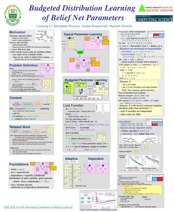
1. Budgeted Distribution Learning of Belief Net Parameters A A 0 0 1 1 B B B A R R R • Costs • $ 4 • $18 • $ 5 • $ 5 • Res $12 Remaining Budget: $30 $26 $21 $16 $12 $0 R R probability   Liuyang Li,Barnabas Poczos,Csaba Szepesvari, Russell Greiner • Motivation • Bayesian networks (BNs) • model of a joint distr’n • used in many applications… • How to GET the BN? • Hand-engineer BNs? • Requires person to KNOW the structure, parameters… Learn BNs from data • Most models assume data are available initially… • but might not be available initially • data can be costly to obtain (time, energy, ...) • Medical tests can be very expensive! Typical Parameter Learning • Proposition: When independent: • Loss Function decomposesJ( A ) = iJi( Ai) • Ji( Ai) just depends on size of Ai| Ai | = | Ai’| Ji( Ai) = Ji( Ai ’) • So viewJi( Ai) = Ji( |Ai|) = Ji( k) • Ji(.) for Xi ~ Bernoulli() and  ~ Beta(,) is Monotone non-increasing and Supermodular • Monotone: A  A’J( A ) J( A ’) • Supermodular: A  A’ J( A )– J( A  {v}) J( A’)– J( A’ {v}) • Let i(k) = Ji(k) – Ji(k+1)… always positive, & smaller with increasing k… • True for Beta/Bernoulli variables! • Need to computei(k+1)fromi(k): • For Beta priors, requires O(k) time • IGA requires O( (n’+B)B ln n’) time, O(n’) space • cmin  min{ ci }; n’ = n / cmin Response Patient 1 Patient 2 Learner • Problem Definition • Given • structure of belief net; prior over parameters • no initial data, but … • budget B+to use to acquire data • Collect data by performing sequence of probes • Probe dij obtains value of attribute i for patient j … at cost ci • Cost of K probes is • After spending B, use data to estimate model parameters • Goal: an accurate generative model of the joint distribution over the features IGA( budget B; costs ci; reductions i(k) ) s = 0 ; a1= a2 = … = an = 0 while s < B do j* := arg maxj { i(aj) / cj} aj* += 1; s += cj* return [ a1, …, an ] R Budgeted Parameter Learning Theorem: If • all cis are equal • all Ji(.)s are monotone and supermodular Then IGA computes optimal allocation. Total Budget: $30 Response Patient 1 Patient 2 • Context BGL: BudgetedGenerative(-) Learning • Given nothing about training instances, • pay for any feature [no “labels”, no “attributes” ] • to produce generative model • … subject to fixed total $$ Label Attribute – Active Budgeted Discriminative Generative Learning • Loss Function • R.v. X ~ Pr( . | ) • Parameter-tuple induces distr’n of X • Recall ~p(.) • Single estimate: Mean: E[ ]=  • For any parameter value , loss of using  when should use  is: KL(|| ) = xX Pr(x | ) ln[Pr(x | ) / Pr(x | ) ] • Don’t know  … so averageJ( p(.) ) = E~p(.)[ KL(|| E[] ) ] • Set of probes: A= { (A,1), (D,1), (D,2), (A,2), (E,1) } • XA = values returned (r.v.) • (A,1,b), (D,1,x), (D,2,+), (A,2,a), (E,1,0) • XA=E[|XA]=“mean parameter values”, wrt XA • J( A ) = Loss of posterior, based on probes A = E~p(.)EXA~ Pr(. | )[ KL(|| XA) ] Theorem: It is NP-hard to compute budgeted allocation policy that minimizes J(.) • even if variables are independent • when costs can differ. • RoundRobin: • Instance#1: f1, then f2, then …, then fn, then… • Instance#2: f1, then f2, then …, then fn, then… • Adaptive Greedy Algorithm (AGA): • Probe: arg maxj { i(1) / cj} • Optimal is  O(n) better than AGA • IGA: 1 flip to A and 1 flip to B • AGA: Flip B, and then flip A • Optimal Adaptive: • Empirical studies: • Related Work • IAL: Interventional Active Learning of Generative BNs • [Ton&Koller, 2001a,b]; [Murphy,2001]; [Steck&Jaakkoa,2002] • Learner sets values of certain features (interventions) over all training instances • Learner receives ALL of remaining values of each specified instance • Seeks BN parameters optimizing Generative distribution • Differences: • BGL cannot see (for free) any values: must pay for each probe • BGL has explicit budget • BGL can pay for only some features of instance Label Attribute – Active Budgeted Discriminative Generative Learning Adaptive Dependent + – – + • Foundations • Nodes  r.v.s X • Arcs  dependencies • Parameters  quantify conditional distribution of each variable, given parents • drawn from a distribution  ~ Pr(.) • Here: Variables discrete, distributed as (independent) Beta/Dirichlet Constant Costs Non-Constant Costs IGA, AGA > Random, RoundRobin – Wilcoxon signed rank p<0.05 • Given: • prior is product of Dirichlet dist’ns, • COMPLETE training tuples • Then: • posterior is product of Dirichlet dist’ns • If incomplete training tuples (missing r values): • Then posterior is MIXTURE of O(2r) product of Dirichlet dist’ns • “Complete tuple” fails: • if not complete graph • if not BDE • if not unit cost • GreedyAlg, given partial data • Approximate J(.) … then greedy using this approx (Allocation alg) ?Conjecture? If • BN is complete graph over d variables • parameters have BDE priors • probes have unit cost ci Then: Optimal allocation strategy = collect COMPLETE tuples B=10 S=5 • Holds: • For d=2 ICML 2010, the 27th International Conference on Machine Learning Greedy > Random, RoundRobin – Wilcoxon signed rank p<0.05