Download

1 / 12
160 likes | 408 Vues
Chapter 4 OPTIMIZED IMPLEMENTATION OF LOGIC FUNCTIONS. 4.1 Karnaugh Mapping. Used to minimize the number of gates Reduce circuit cost Reduce physical size Reduce gate failures Requires SOP form Karnaugh Mapping Graphically shows output level for all possible input combinations

E N D
4.1 Karnaugh Mapping • Used to minimize the number of gates • Reduce circuit cost • Reduce physical size • Reduce gate failures • Requires SOP form • Karnaugh Mapping • Graphically shows output level for all possible input combinations • Moving from one cell to an adjacent cell, only one variable changes 31
Karnaugh Mapping • Steps for K-map reduction: • Transform the Boolean equation into SOP form. • Fill in the appropriate cells of the K-map. • Encircle adjacent cells in groups of 2, 4 or 8. • Adjacent means a side is touching, NOT diagonal. • Watch for the wraparound • Find each term of the final SOP equation by determining which variables remain the same within circles. 33
x x 2 1 x x 1 2 0 1 m 0 0 0 m m m 0 1 0 1 0 2 m 1 0 2 m m 1 1 3 m 1 1 3 (a) Truth table (b) Karnaugh map Figure 4.2. Location of two-variable minterms.
1 Figure2.15. The function f (x1, x2) = m(0, 1, 3). Figure 4.3. The function of Figure 2.15.
x x x 1 2 3 x x 1 2 x m 0 0 0 3 0 00 01 11 10 m 0 0 1 1 m m m m 0 0 2 6 4 m 0 1 0 2 m m m m m 0 1 1 1 1 3 7 5 3 m 1 0 0 4 (b) Karnaugh map m 1 0 1 5 m 1 1 0 6 m 1 1 1 7 (a) Truth table Figure 4.4. Location of three-variable minterms.
Figure2.18. The function f (x1, x2, x3) = m(1, 4, 5, 6). x x 1 2 x 3 00 01 11 10 0 0 0 1 1 f x x x x = + 3 2 1 3 1 1 0 0 1 (a) The function of Figure 2.18 Figure 4.5. Examples of three-variable Karnaugh maps.
x x 1 2 x 3 00 01 11 10 0 1 1 1 1 Figure4.1. The function f (x1, x2, x3) = m(0, 2, 4, 5, 6). f x x x = + 3 2 1 1 0 0 0 1 (b) The function of Figure 4.1 Figure 4.5. Examples of three-variable Karnaugh maps.
x x x x 1 2 1 2 x x x x 3 4 3 4 00 01 11 10 00 01 11 10 00 0 0 0 0 00 0 0 0 0 01 0 0 1 1 01 0 0 1 1 11 1 0 0 1 11 1 1 1 1 10 1 0 0 1 10 1 1 1 1 f = x x + x x x 2 3 1 3 1 4 x x x x 1 2 1 2 x x x x 3 4 3 4 00 01 11 10 00 01 11 10 00 1 0 0 1 00 1 1 1 0 01 0 0 0 0 01 1 1 1 0 11 1 1 1 0 11 0 0 1 1 10 1 1 0 1 10 0 0 1 1 f = x + x x 2 3 1 4 x x 1 2 f = x x + x x + x x x f = x x + x x + or 2 4 1 1 3 3 3 2 3 4 4 1 3 x x 3 2 Figure 4.7. Examples of four-variable Karnaugh maps.
Index of 5-variable Karnaugh map x1x2x3x4x5: x5 is the least significant bit. x x x x 1 2 1 2 x x x x 3 4 00 01 11 10 3 4 00 01 11 10 00 1 9 25 17 00 0 8 24 16 01 3 11 27 19 01 2 10 26 18 11 7 15 31 23 11 6 14 30 22 10 5 13 29 21 10 4 12 28 20 (b) (a)