Download

1 / 48
580 likes | 1.78k Vues
HFSS 的后处理及场计算器入门. 电子科技大学 贾宝富. Ansoft HFSS 的后处理( Results ). Create Report. 可绘制图形. Eigenmode solution (本征模解) Eigenmode Parameters (modes) (本征模参数图形) Driven Modal Solution (驱动模式解) S-parameters ( S 参数图形) Y-parameters ( Y 参数图形) Z-parameters ( Z 参数图形) VSWR (驻波比)

E N D
HFSS的后处理及场计算器入门 电子科技大学 贾宝富
Ansoft HFSS的后处理(Results) • Create Report
可绘制图形 • Eigenmode solution(本征模解) • Eigenmode Parameters (modes)(本征模参数图形) • Driven Modal Solution(驱动模式解) • S-parameters(S参数图形) • Y-parameters(Y参数图形) • Z-parameters(Z参数图形) • VSWR(驻波比) • Gamma (complex propagation constant)(复数形式的传播常数) • Port Zo(端口波阻抗) • Driven Terminal Solution(终端驱动解) • S-parameters(S参数图形) • Y-parameters(Y参数图形) • Z-parameters(Z参数图形) • VSWR(驻波比) • Power(功率) • Voltage Transform matrix (T)(电压传输矩阵) • Terminal Port Zo(端口波阻抗)
可绘制图形 • Fields(场) • Mag_E • Mag_H • Mag_Jvol • Mag_Jsurf • ComplexMag_E • ComplexMag_H • ComplexMag_Jvol • ComplexMag_Jsurf • Local_SAR (Specific Absorption Rate) • Average_SAR • 注:在绘制场图前必须先选择一个面或者一个多点线。
Ansoft HFSS的后处理(Results) • Solution Data
Ansoft HFSS的后处理(Results) • Output Variables
Ansoft HFSS的后处理(Fields) • Fields
Ansoft HFSS的后处理(Radiation) • Radiation
What is Time Domain Reflectometry? • Time Domain Reflectometry (TDR) measures the reflections that result from a signal travelling through a transmission environment of some kind – a circuit board trace, a cable, a connector and so on. • The TDR instrument sends a pulse through the medium and compares the reflections from the unknown transmission environment to those produced by a standard impedance.
The Reflection Coefficient • TDR measurements are described in terms of a Reflection Coefficient, (rho). The coefficient r is the ratio of the reflected pulse amplitude to the incident pulse amplitude:
Calculating the Impedance of the Transmission Line and the Load
HFSS Field Calculator: Definition • A tool for performing mathematical operations on ALLsaved field data in the modeled geometry • E,H,J, and Poynting data available • Perform operations using drawing geometry or new geometry created in Post3 • Perform operations at single frequency (interpolating or discrete sweeps) or other frequencies (fast sweep) • Generate numerical , graphical, geometrical or exportable data • Macro-enabled
场计算器分区 指定数据关联 表达式操作区 场计算器操作区
表达式操作区 • 建立表达式 • 使用“Add”键,由场计算器堆栈导入表达式; • 使用“Load From”键,由场计算器表达式文件(*.clc)导入表达式; • 输出表达式 • 使用“Copy to stack”键,将已存在的表达式导出到场计算器堆栈; • 使用“Save to”键,将已存在的表达式保存成场计算器表达式文件(*.clc) ;
指定关联区 • 指定场计算器使用数据的出处。 • 指定求解设置 • 指定场类型; • 指定频率 • 指定相位
HFSS Field Calculator: Basic Layout Data stack: Contains current and saved entries in a scrolling stack similar to a hand-held scientific caculator. Stack Operations: Button for manipulating stack Calculator Functions: Orgnized groupings of all the avaliable calculator functions in button format. Some buttons contain further options as drop-down menus Status Bar(not currently shown):
HFSS Field Caculator: Data Types • The calculatiorv can manipulate many different types of data • Geometric • Complex • Vector • Scalar • Data types are indicated in the calculator stack for each entry • Most calculator operations are only available on the appropriate data type(s) Geometric surface generated along E field iso-value contour Vector data output to a plane geometry Scalar E-field data graphed along a line geometry
HFSS Field Calculator: Data Indicators • Each stack entry will be preceded by a unique code denoting its data type • Mathematical: • CVc: Complex Vector • Vec: Vector • CSc: Complex Scalar • Scl: Scalar • Geometric: • Pnt: Point • Lin: Line • Srf: Sourface • Vol: Volume • Combinations can also exist • E.g. “SclSrf”: Scalar data distributed on a Surface geometry CACULATOR USAGE HINT: Most data input types will be self-explanatory, e. g. E and H fields being phasor quantities will be Complex Vector (CVc). The only exception to this rule is the Poynting input, Which will show up as a “CVc” even though E X H* should have no imaginary component. The calculator only knows that two complex vector were crossed, and does not know ahead of time that the imaginary component has been zeroed.
HFSS Field Calculator: Detail Layout-Stack UNDO attempts to take back the last operation between stack enties. It may not work for all data types (e.g. the result of a pure math operation cannot be reversed) As data is entered into the calculator it appears at the TOP of the stack, pushing older entries DOWN PUSH duplicates the top stack entry CLEAR deletes ALL entries from the stack upon confirmation POP deletes the top entry off the stack EXCH exchanges or swaps the top two stack entries RLDN “rolls” the stack downward, moving the top entry to the bottom RLUP “rolls” the stack upward, moving the bottom entry to the top
HFSS Field Calculator: Detail Layout-Operations SCALAR column operations can only be performed on Scalar data (not complex or vector data), such as finding the Cosine of a value using the trig functions. OUTPUT column operations result in the generation of calculator outputs, in either numerical, graphical (displayed as 2D graphs or in the 3Dview), or exported form. INPUT column contain all operations which input new data into the stack (field data, constant, user-entered vector or complex numbers, etc. VECTOR column contains operations to be performed on vector data such as converting to scalar, Dot and Cross products,and Unit Vector computations All calculator operations are orgnized into columns classifyying them by the type of operation and the type of the data upon which the operation can be performed. GENERAL column contains operations which can be performed on many data types (e. g. adding scalar values or adding vectors)
HFSS Field Calculator: Usage-Overview • Use just like a scientific calculator • Similar to HP scientific calculators • “First Quantity”, ”Second Quantity” Then “Operation” • Remember stack fills from the Top and pushes older contents below. • General use progresses from left to right • Input quantity or quantities at left • Perform operations in middle • Operate between quantities; apply quantities to geometries, etc. • Define desired output type at right. Calculator Usage HINT:Any Time you use the field post –processor to plot a quantity (PlotFields), you are actually performing operations using the calculator!! To see the steps that went into the generating the plot you just created, open the calculator interface and view the stack contents. This can often help guide you as you try to use the calculator to created your own custom outputs.
HFSS Field Calculator: Usage-Changing Data Types • As discussed previously, Many operations must be on the correct data type. • Many operations result in a different data type than the inputs. • Ex1:The Dotproduct of two Vector is a Scalar. • Ex2:Obtaining the Unit VecNormal to a Surf Generates a Vector. • Some calculator buttons exist primarily to assist in type conversion. • Vec? Converts Scl to Vec data • Scal? Does the reverse • CmplxReal or CmplxImag takes a Scl component from a CSc or CVc. • CmplxCmplxR or CmplxCmplxI take a Vec or Scl component and make it the real or imaginary part of a complex value CVc or CSc, respectively. Always think of what type of data you are working with and whether or not it is compatible with your desired operation .For example, not the INTEGRAL sign is in the Scalar column, implying that to integrate complex numbers you will have to integrate the real and imaginary components separately, performing an integration by parts.
HFSS Field Calculator: Usage-Input Types • The available field inputs are • E: The complex vector E field data everywhere in the modeled geometry; • H: The complex vector H field data everywhere in the modeled geometry; • Poynting: The time-average Poynting vector computed from above as (E×H*): • Jvol: Current density in a volume, computed as (σ+jωε”)E which contain both conduction and displacement current ; • Jsurf: Net surface current computed as n×(H|top tetrahedra- H|bottom tetrahedra): • Unlike other quantities, Jsurf can only be output on an object surface geometry. E H Jsurf Jvol Poynting E and H are Peak Phasor representation of the steady state fields. Therefore the current representation J derived from n×H or σE are also peak phasor quantities. The Poynting Vector input is a time-averaged quantity.
HFSS Field Calculator: Usage-Output Types • Different data output can be generated depending on selected Output column button and stack content(s): • Value is used to take the “value” of a field stack entry on a specific geometry; • Eval turn stack placeholder text into final numerical answer; • Write and Export outputs stack data to output file formats for use outside the calculator or current project.
HFSS Field Calculator: Usage-Possible Operations • As long as you can perform the math using the interface, there is no restriction on the possible calculator operations available: • Outputs derived can be other than “Electromagnetic” in nature; • Pure Geometric operations (vector and surface cross and dot products, generation of iso-surface contours from any scalar data field imported into the geometry, etc) • Thermal heating computations derived from field values combined with thermal mass characteristics and equations; • Integrations to obtain summary quantities such as Quanlity factors, power dissipation or flux,etc.
Post-Processor Exercise : Helix Interaction Impedance: Calculating Point βZ= 2π / λg λg= vp / f Cut Plane
定向耦合器 混合电桥 滤波器 对称 非对称 可用于设计各类器件 耦合带状线及耦合微带线 (coupled stripline and coupled microstrp line) 耦合传输线:两根或多根彼此靠的很近的非屏蔽传输线系统
2. 耦合线理论与奇耦模分析方法 耦合形式分为: 常用的耦合微带线是侧边耦合对称耦合微带线
<1> 奇耦模分析方法——利用对称性 ( odd/even excitation methods ) V=0 奇模激励(odd-mode excitation): 大小相同,方向相反的电流对耦合线两导带的激励(中心电壁) 偶模激励(even-mode excitation): 大小相同,方向相同的电流对耦合线两导带的激励(中心磁壁) -V V H=0
描述传输线的基本参数 • 传播常数: • 衰减常数; • 相位常数 • 相位速度 • 波长 • 特性阻抗
奇模相速度、奇模波导波长和奇模特性阻抗 耦合系数 奇模阻抗 单线特性阻抗 双线特性阻抗
偶模相速度、偶模波导波长和偶模特性阻抗 偶模阻抗
耦合系数的分贝耦合度为: 均匀填充介质的对称线 4.3-25