Download
1 / 19
190 likes | 199 Vues
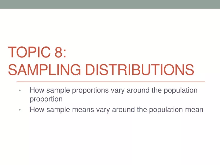
Topic 8: Sampling Distributions. How sample proportions vary around the population proportion How sample means vary around the population mean. Populations and samples. We are often interested in population parameters .

E N D
Topic 8: Sampling Distributions How sample proportions vary around the population proportion How sample means vary around the population mean
Populations and samples • We are often interested in population parameters. • Since complete populations are difficult (or impossible) to collect data on, we use sample statistics as point estimates for the unknown population parameters of interest. • Sample statistics vary from sample to sample. • Quantifying how sample statistics vary provides a way to estimate the margin of error associated with our points estimate. • For this topic, let’s try to understand how point estimates vary from sample to sample. Suppose we randomly sample 1,000 adults from each state in the US. Would you expect the sample means of their heights to be the same, somewhat different, or very different?
Populations and samples • We are often interested in population parameters. • Since complete populations are difficult (or impossible) to collect data on, we use sample statistics as point estimates for the unknown population parameters of interest. • Sample statistics vary from sample to sample. • Quantifying how sample statistics vary provides a way to estimate the margin of error associated with our points estimate. • For this topic, let’s try to understand how point estimates vary from sample to sample. Suppose we randomly sample 1,000 adults from each state in the US. Would you expect the sample means of their heights to be the same, somewhat different, or very different? Not the same, but only somewhat different.
How sample proportions vary around the population proportion
Example: do you smoke? 30,000 college students were asked if they smoke. Their answers are summarized below. 25.87% of the college students reported that they smoke.
Example: do you smoke? 30,000 college students were asked if they smoke. Their answers are summarized below. 25.87% of the college students reported that they smoke. Suppose this is our population, and we want to estimate this percentage by choosing a sample.
A random sample of 1000 students Our statistic: 27.60% (proportion of 1000 randomly selected students that smoke) Parameter: 25.87% (proportion of all 30,000 students that smoke).
A random sample of 1000 students Our statistic: 27.60% (proportion of 1000 randomly selected students that smoke) Parameter: 25.87% (proportion of all 30,000 students that smoke). Our statistic is quite close. Were we lucky, or is there a reason?
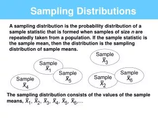
Sampling Distribution We repeatedly take a random sample of 1000 students and compute the statistic (proportion that smoke). Below is a histogram displaying the statistics computed for many samples.
Sampling Distribution We repeatedly take a random sample of 1000 students and compute the statistic (proportion that smoke). Below is a histogram displaying the statistics computed for many samples. Mean = .2583 Standard Deviation = 0.0140
The central limit theorem (proportions) The distribution of the sample proportion is well approximated by the normal model: Where p is the population proportion and n in the sample size. SE is the standard error, which is the standard deviation of the sampling distribution. • It wasn’t coincidence that our sample proportion was “close” to the population proportion. • It wasn’t coincidence that the sampling distribution was centered at the population proportion and approximately normal. • Note: if the sample size increases, then the standard error decreases.
Central limit theorem (CLT): conditions for proportions Certain conditions must be met for the CLT to apply: • We have a random sample from the population • The sample is large enough so that we see at least 5 observations of both possible outcomes
Example: what do MLB players make? The salaries of 16,383 Major League Baseball players are displayed in the histogram below. Mean salary for these players is $1,265,466 Suppose this is our population, and we want to estimate this mean by choosing a small sample.
A random sample of 1000 players The salaries of 1,000 Major League Baseball players are displayed in the histogram below. Our statistic: $1,261,780.70 (mean salary of randomly selected 1,000 players) Parameter: $1,265,466 (mean salary for all 16,383 players). Our statistic is quite close. Again, were we lucky or is there a reason?
Sampling Distribution We repeatedly take a random sample of 1000 players and compute the statistic (mean salary). Below is a histogram displaying the statistics computed for many samples.
Sampling Distribution We repeatedly take a random sample of 1000 players and compute the statistic (mean salary). Below is a histogram displaying the statistics computed for many samples. Mean = $1,266,084.20 Standard deviation = $66,220.87
The central limit theorem (means) The distribution of the sample mean is well approximated by the normal model: Where μ is the population mean and n in the sample size. SE is the standard error, which is the standard deviation of the sampling distribution. • It wasn’t coincidence that our sample mean was “close” to the population mean. • It wasn’t coincidence that the sampling distribution was centered at the population mean and approximately normal. • Note: if the sample size increases, then the standard error decreases.
Central limit theorem (CLT): conditions for means Certain conditions must be met for the CLT to apply: • The more skewed the population distribution, the larger sample size we need for CLT to apply. • For moderately skewed distributions n > 30 is a widely used rule of thumb.