Download
1 / 42
470 likes | 759 Vues
Information and Coding Theory. Dr Costas Constantinou School of Electronic, Electrical & Computer Engineering University of Birmingham W: www.eee.bham.ac.uk/ConstantinouCC/ E: c.constantinou@bham.ac.uk. Recommended textbook.

E N D
Information and Coding Theory Dr Costas Constantinou School of Electronic, Electrical & Computer Engineering University of Birmingham W: www.eee.bham.ac.uk/ConstantinouCC/ E: c.constantinou@bham.ac.uk
Recommended textbook • Simon Haykin and Michael Moher, Communication Systems, 5th Edition, Wiley, 2010; ISBN:970-0-470-16996-4
Information theory • Claude E Shannon (1948) A Mathematical Theory of Communication, The Bell System Technical Journal, Vol. 27, pp. 379–423, 623–656, July, October • How to describe information sources • How to represent information from a source • How to transmit information over a channel
Information sources • Consider the following forecast: • Birmingham on 15 July at midday; cloudy • Birmingham on 15 July at midday; sunny • The forecast is an information source; the information has two outcomes, cloudy and sunny • Now consider the following forecast: • Cairo on 15 July at midday; cloudy • Cairo on 15 July at midday; sunny • This forecast is another information source; the information also has two outcomes, cloudy and sunny. Since we expect it to be sunny, the latter outcome has little information since it is a highly probable outcome; conversely the cloudy contains a lot of information since it is highly improbable outcome
Information sources • The information content, I, of an outcome (or information symbol), xi, occurring with probability, pi, must obey the following properties:
Information sources • A measure of the information contained in an outcome and satisfying all of the earlier properties was introduced by Hartley in 1927 • Hartley defined the information (sometimes called self-information) contained in an outcome, xi, as,
Information sources • The choice of the logarithm base 2, and the arbitrary multiplicative constant of 1, simply give the unit of information, in this case the bit • Choosing a logarithm base of 10 gives the unit of Hartley • Choosing a logarithm base of e (natural logarithms) gives the unit of nat • Hartley's measure defines the information in a single outcome – we are interested in the information content of a source
Information sources • The measure entropy, H(X), defines the information content of the source X as a whole • It is the mean information provided by the source per outcome, or symbol • It is measured in bits/symbol • A binary symmetric source (BSS) is a source with two outputs whose probabilities are p and 1 – p respectively
Information sources • The weather forecast we discussed earlier is a BSS • The entropy of this information source is: • When either outcome becomes certain (p = 0 or p= 1), the entropy takes the value 0 • The entropy becomes maximum when p= 1 – p = ½
Information sources • An equiprobable BSS has an entropy, or average information content per symbol, of 1 bit per symbol • Warning: Engineers use the word bit to describe both the symbol, and its information content [confusing] • A BSS whose outputs are 1 or 0 has an output we describe as a bit • The entropy of the source is also measured in bits, so that we might say the equi-probable BSS has an information rate of 1 bit/bit • The numerator bit refers to the information content; the denominator bit refers to the symbol 1 or 0 • Advice: Keep your symbols and information content units different
Information sources • For a BSS, the entropy is maximised when both outcomes are equally likely • This property is generally true for any number of symbols • If an information source X has k symbols, its maximum entropy is log2k and this is obtained when all k outcomes are equally likely • Thus, for a k symbol source: • The redundancy of an information source is defined as,
Information sources • Redundancy – natural languages • A natural language is that used by man, in spoken or written form, such as, English, French, Chinese • All natural languages have some redundancy to permit understanding in difficult circumstances, such as a noisy environment • This redundancy can be at symbol (letter) level, or word level • Here we will calculate redundancy at symbol level
Information sources • The maximum entropy occurs when all symbols have equal probability • Thus in English, with 27 letters plus a space, • Assuming the symbols/letters in the English language are independent and their frequencies are given in the table, Note: H is really much smaller, between 0.6 and 1.3, as listeners can guess the next letter in many cases
Source coding • It is intuitively reasonable that an information source of entropy H needs on average only H binary bits to represent each symbol • The equiprobable BSS generates on average 1 information bit per symbol bit • Consider the Birmingham weather forecast again: • Suppose the probability of cloud (C) is 0.1 and that of sun (S) 0.9 • The earlier graph shows that this source has an entropy of 0.47 bits/symbol • Suppose we identify cloud with 1 and sun with 0 • This representation uses 1 binary bit per symbol • Thus we are using more binary bits per symbol than the entropy suggests is necessary
Source coding • The replacement of the symbols rain/no-rain with a binary representation is called source coding • In any coding operation we replace the symbol with a codeword • The purpose of source coding is to reduce the number of bits required to convey the information provided by the information source (reduce redundancy) • Central to source coding is the use of sequences • By this, we mean that codewords are not simply associated to a single outcome, but to a sequence of outcomes • Suppose we group the outcomes in threes (e.g. for 15, 16 and 17 July), according to their probability, and assign binary codewords to these grouped outcomes
Source coding • The table here shows such a variable length code and the probability of each codeword occurring for our weather forecasting example • It is easy to compute that this code will on average use 1.2 bits/sequence • Each sequence contains three symbols, so the code uses 0.4 bits/symbol
Source coding • Using sequences decreases the average number of bits per symbol • We have found a code that has an average bit usage less than the source entropy – how is this possible? • BUT, there is a difficulty with the previous code: • Before a codeword can be decoded, it must be parsed • Parsing describes the activity of breaking a message string into its component codewords • After parsing, each codeword can be decoded into its symbol sequence • An instantaneously parseable code is one that can be parsed as soon as the last bit of a codeword is received • An instantaneous code must satisfy the prefix condition: No codeword may be a prefix of any other codeword • This condition is not satisfied by our code • The sequence 011 could be 0-11 (i.e. SSS followed by CCS) or 01-1 (i.e. SCS followed by SSC) and is therefore not decodable unambiguously
Source coding • The table here shows an instantaneously parseable variable length code and it satisfies the prefix condition • It is easy to compute that this code uses on average 1.6 bits/sequence • The code uses 0.53 bits/symbol • This is a 47% improvement on identifying each symbol with a bit • This is the Huffman code for the sequence set
Source coding • The code for each sequence is found by generating the Huffman code tree for the sequence • A Huffman code tree is an unbalanced binary tree • The derivation of the Huffman code tree is shown in the next slide • STEP 1: Have the n symbols ordered according to non-increasing values of their probabilities • STEP 2: Group the last two symbols xn-1 and xn into an equivalent “symbol” with probability pn-1 + pn • STEP 3: Repeat steps 1 and 2 until there is only one “symbol” left • STEP 4: Looking at the tree originated by the above steps (see next slide), associate the binary symbols 0 and 1 to each pair of branches at each intermediate node – the code word for each symbol can be read as the binary sequence found when starting at the root of the tree and reaching the terminal leaf node associated with that symbol
Source coding (0.729) (0.081) (0.271) (0.109) (0.081) (0.081) (0.081) (0.162) (0.081) (0.109) (0.028) (0.010) (0.009) (0.009) (0.018) (0.010)
Source coding 1 0 SSS STEP 4 1 0 (1) 0 0 1 1 SSC SCS CSS 1 (010) (011) (001) 0 0 1 0 1 SCC CCC CCS CSC (00001) (00011) (00010) (00000)
Source coding • Huffman coding relies on the fact that both the transmitter and the receiver know the sequence set (or data set) before communicating and can build the code table • The noiseless source coding theorem (also called Shannon’s first theorem) states that an instantaneous code can be found that encodes a source of entropy, H(X), with an average number of bits per symbol, Bs, such that, • The longer the sequences of symbols, the closer Bs will be to H(X) • The theorem does not tell us how to find the code • The theorem is useful nevertheless: in our example, the Huffman code uses 0.53 bits/symbol which is only 11% more than the best we can do (0.47 bits/symbol)
Communication channels • A discrete channel is characterised by an input alphabet, X, and output alphabet, Y, and a set of conditional probabilities, pij = P(yj|xi) • We assume that the channel is memoryless, i.e. for a binary channel (BC), P(y1,y2| x1,x2) = p11p12p21p22
Communication channels • The special case of the binary symmetric channel (BSC) is of particular interest, i.e. p12 = p21 = p • For the BSC, the probability of error is,
Communication channels • We now have a number of entropies to consider: • Input entropy, which measures the average information content of the input alphabet • Output entropy, which measures the average information content of the output alphabet
Communication channels • The joint entropy, which measures the average information content of a pair of input and output symbols, or equivalently the average uncertainty of the communication system formed by the input alphabet, channel and output alphabet as a whole
Communication channels • The conditional entropy, H(Y|X), which measures the average information quantity needed to specify the output symbol when the input symbol is known • The conditional entropy, H(X|Y), which measures the average information quantity needed to specify the input symbol, when the output or received symbol is known • H(X|Y) is the average amount of information lost in the channel and is called equivocation
Communication channels • The following relationships between entropies hold • The information flow through, or mutual information of thechannel is defined by, • Therefore, • The capacity of a channel is defined by
Communication channels • Making use of • Combining this with the expression for H(X|Y), gives,
Communication channels • In the case of a BSC, I(X;Y) is maximised when H(X) is maximised, i.e. when P(x1) = P(x2) = ½ • For a BSC, we have, • Direct substitution of the above transition probabilities into the last expression for I(X,Y), and making use of Baye’s theorem, P(xi,yj) = P(yj|xi)P(xi) = P(xi|yj)P(yj), gives,
Communication channels • We can now see how the BSC capacity varies as a function of the error or transition probability, p • When the error probability is 0, we have a maximum channel capacity, equal to the binary symmetric source information content • When the error probability is 0.5, we are receiving totally random symbols and all information is lost in the channel
Channel coding • Source coding represent the source information with the minimum of symbols – minimises redundancy • When a code is transmitted over an imperfect channel (e.g. in the presence of noise), errors will occur • Channel coding represents the source information in a manner that minimises the error probability in decoding • Channel coding adds redundancy
Channel coding • We confine our attention to block codes: we map each k-bit block to a n-bit block, with n > k, e.g.: • 00 to 000000 • 01 to 101010 • 10 to 010101 • 11 to 111111 • The Hamming distance between codewords is defined as the number of bit reversals required to transform one codeword into another • The Hamming distance of the above code is 3 • If the probability of bit error (1 bit reversal) is 0.1, then when we receive 000100 we know with a certainty of 99% that 000000 was sent
Channel coding • The ratio r = k/n is called the code rate • Can there exist a sophisticated channel coding scheme such that the probability that a message bit will be in error is less than an arbitrarily small positive number? • The source emits one symbol per TS seconds, then its average information rate is H/TS bits per second • These symbols are transmitted through a discrete memoryless channel of capacity C and the channel can be used once every TC seconds
Channel coding • Shannon’s channel coding theorem (2nd theorem) states that: • If H/TSC/TC there exists a coding scheme with an arbitrarily small probability of error (equality implies signalling at the critical rate) • If H/TS>C/TC it is not possible to transmit information over the channel and reconstruct it with an arbitrarily small probability of error • For a BSC, • H = 1 • r = k/n = TC/TS • Shannon’s channel coding theorem can be restated as, if rC there exists a code with this rate capable of arbitrarily low probability of error
Capacity of a Gaussian channel • Band-limited, power-limited Gaussian channels • Transmitted signal • Signal is random process, X(t) • Signal is sampled at Nyquist rate of 2B samples per second • Let Xk, k = 1, 2, 3, ..., Kdenote the samples of the transmitted signal • Signal samples are transmitted over noisy channel in T seconds • Hence, K = 2BT • Finally, we assume that the transmitted signal is power limited, E[Xk2] = P, being the averagetransmittedpower
Capacity of a Gaussian channel • Noise • Channel is subject to additive white Gaussian noise of zero mean and power spectral density N0/2 • Noise is also band-limited to B Hz • The noise sample Nk is therefore Gaussian with zero mean and variance s2 = N0B • Received signal • The samples of the received signal are Yk = Xk + Nk • We assume that Yk are statistically independent
Capacity of a Gaussian channel • The information capacity of this channel is • Performing the maximisation w.r.t.fXk(x), the probability density function of Xk, (difficult calculation omitted in this introductory module), gives,
Capacity of a Gaussian channel • Since the channel is used K times for the transmission of K samples of X(t) in T seconds, the information capacity per unit time is (K/T) times the previous result, with K = 2BT • This is a fundamental limit on the rate of error-free transmission for a power-limited, band-limited Gaussian channel
Capacity of a Gaussian channel • Implications of the information capacity theorem • Assume we have an ideal system, defined as one that transmits data at a bit rate Rb = C • The average transmit power is P = EbC • The we can re-write the information capacity equation as
Capacity of a Gaussian channel • Infinite bandwidth case • Capacity boundary divides the region that can support error-free transmission from the region that cannot (shaded) • Trade-offs among Eb/N0, Rb/B, and P(e) can be visualised on the graph