Download
1 / 62
620 likes | 746 Vues
Relational Database Theory. Designing high quality tables. Remove redundancy! Decomposition! How can decomposition be no error ? How to determine the primary key?. Functional Dependency (1).

E N D
Relational Database Theory Designing high quality tables. Remove redundancy! Decomposition! How can decomposition be no error ? How to determine the primary key?
Functional Dependency (1) Definition: Let R(A1, ..., An) be a relation schema. Let X and Y be two subsets of {A1, ..., An}. X is said to functionally determine Y (or Y is functionally dependent on X) if for every legal relation instance r(R), for any two tuples t1 and t2 in r(R), we have t1[X] = t2[X] t1[Y] = t2[Y].
Functional Dependency (2) Two notations: • X R denotes that X is a subset of the attributes of R. • X Y denotes that X functionally determines Y.
Functional Dependency (3) Several equivalent definitions: • X Y in R for any t1, t2 in r(R), if t1 and t2 have the same X-value, then t1 and t2 also have the same Y-value. • X Y in R there exist no t1, t2 in r(R) such that t1 and t2 have the same X-value but different Y-values. • X Y in R for each X-value, there corresponds to a unique Y-value.
Functional Dependency (4) Theorem 1: If X is a superkey of R and Y is any subset of R, then X Y in R. • Note that X Y in R is a property that must be true for all possible legal r(R), not just for the present r(R).
Functional Dependency (5) Example: which is true? A B C D A B a1 b1 c1 d1 A C a1 b2 c1 d2 C A a2 b2 c2 d2 A D a2 b3 c2 d3 B D a3 b3 c2 d4 AB D
Identify Functional Dependency (1) • Trivial FDs: if Y X R, then X Y. • A special case: for any attribute A, A A. • Use Theorem 1: If X is a superkey of R and Y is any subset of R, then X Y is in R.
Identify Functional Dependency (2) • Created by assertions. Employees(SSN, Name, Years_of_emp, Salary, Bonus) Assertion: Employees hired the same year have the same salary. This assertion implies: Years_of_emp Salary
Identify Functional Dependency (3) • Analyze the semantics of attributes of R. Addresses(City, Street, Zipcode) Zipcode City • Derive new FDs from existing FDs. Let R(A, B, C), F = {A B, B C}. A C can be derived from F. Denote F logically implies A C by F |= A C.
Identify Functional Dependency (4) Definition: Let F be a set of FDs in R. The closure of F is the set of all FDs that are logically implied by F. • The closure of F is denoted by F+. F+ = { X Y | F |= X Y}
Identify Functional Dependency (5) • A BIG F+ may be derived from a small F. Example: For R(A, B, C) and F = {A B, B C} F+ = { A B, B C, A C, A A, B B, C C, AB AB, AB A, AB B, ... } |F+| > 30.
Computation of F+ (1) Armstrong's Axioms (1974): (IR1) Reflexivity rule: If X Y, then X Y. (IR2) Augmentation rule: { X Y } |= XZ YZ. (IR3) Transitivity rule: { X Y, Y Z } |= X Z.
Computation of F+ (2) Theorem: Armstrong's Axioms are sound and complete. Sound --- no incorrect FD can be generated from F using Armstrong's Axioms. Complete --- Given a set of FDs F, all FDs in F+ can be generated using Armstrong's Axioms.
Computation of F+ (3) Additional rules derivable from Armstrong's Axioms. (IR4) Decomposition rule: { X YZ } |= { X Y, X Z } (IR5) Union rule: { X Y, X Z } |= X YZ (IR6) Pseudotransitivity rule: { X Y, WY Z } |= WX Z
Computation of F+ (4) (IR4): { X YZ } |= { X Y, X Z } Proof: by (IR1): YZ Y, YZ Z; by X YZ, YZ Y and (IR3): X Y; by X YZ, YZ Z and (IR3): X Z.
Computation of F+ (5) (IR5): { X Y, X Z } |= X YZ Proof: by X Y and (IR2): XX XY, i.e., X XY; by X Z and (IR2): XY ZY; by X XY, XY ZY and (IR3): X YZ.
Computation of F+ (6) (IR6): { X Y, WY Z } |= WX Z Proof: by X Y and (IR2): XW YW; by WX WY, WY Z and (IR3): WX Z. Claim: If X R and A, B, ..., C are attributes in R, then X A B ... C { X A, X B, ..., X C }
Closure of Attributes (1) How to determine if F |= X Y is true? Method 1: Compute F+. If X Y F+, then F |= X Y; else F |= X Y. Problem: Computing F+ could be very expensive! Consider F = { A B1, ..., A Bn}. Claim: |F+| > 2n. Reason: {A X | X {B1, ..., Bn}} F+.
Closure of Attributes (2) Method 2: Compute X+ : the closure of X under F. X+ denotes the set of attributes that are functionally determined by X under F. X+ = { A | X A F+ } Theorem: X Y F+ if and only if Y X+. Proof: Use the decomposition rule and the union rule.
Algorithm for Computing X+ (1) Input: a set of FDs F, a set of attributes X in R. Output: X+ (= xplus). begin xplus := X; repeat for each FD Y Z in F do if Y xplus then xplus := xplus Z; until no change to xplus; end
Algorithm for Computing X+ (2) Example: R(A, B, C, G, H, I) = ABCGHI X = AG F = {A B, CG HI, B H, A C } Compute (AG)+. Initialization: xplus := AG;
Algorithm for Computing X+ (3) 1st iteration: consider A B, since A is a subset of xplus, xplus = ABG; consider CG HI, since CG is not a subset of xplus, xplus = ABG; consider B H, since B is a subset of xplus, xplus = ABGH; consider A C, since A is a subset of xplus, xplus = ABCGH; (xplus is changed from AG to ABCGH)
Algorithm for Computing X+ (4) 2nd iteration: consider A ---> B, since A is a subset of xplus, xplus = ABCGH; consider CG ---> HI, since CG is a subset of xplus, xplus = ABCGHI; consider B ---> H, since B is a subset of xplus, xplus = ABCGHI; consider A ---> C, since A is a subset of xplus, xplus = ABCGHI; (xplus is changed from ABCGH to ABCGHI)
Algorithm for Computing X+ (5) 3rd iteration: (consider each FD in F again, but there is no change to xplus, exit) Result: (AG)+ = ABCGHI. • The performance of the algorithm is sensitive to the order of FDs in F.
Algorithm for Computing X+ (6) Theorem: Given R(A1, ..., An) and a set of FDs F in R, K R is a • superkey if K+ = {A1, ..., An}; • candidate key if K is a superkey and for any proper subset X of K, X+{A1, ..., An}.
Algorithm for Computing X+ (7) Continue the above example: • AG is a superkey of R since (AG)+ = ABCGHI. • Since A+ = ABCH, G+ = G, neither A nor G is a superkey. • Hence, AG is a candidate key
Relation Decomposition (1) Definition: Let R be a relation schema. A set of relation schemas {R1, R2, ..., Rn} is a decomposition of R if R = R1 ... Rn. Claim: If {R1, R2, ..., Rn} is a decomposition of R and r is an instance of R, then r R1(r) R2(r) . . . Rn(r) Information may be lost (i.e. wrong tuples may be added) due to a decomposition.
Relation Decomposition Consider : SL(Sno, Sdept, Sloc) F={ Sno→Sdept,Sdept→Sloc,Sno→Sloc} How to decomposed the table? Three ways
Relation Decomposition SL ────────────────── Sno Sdept Sloc ────────────────── 95001 CS A 95002 IS B 95003 MA C 95004 IS B 95005 PH B ──────────────────
Relation Decomposition 1. Decompose it into: SN(Sno) SD(Sdept) SO(Sloc)
Result: SN────── SD ────── SO ────── Sno Sdept Sloc ────── ────── ────── 95001 CS A 95002 IS B 95003 MA C 95004 PH ───── 95005 ────── ──────
Relation Decomposition Information lost ! After the decomposition we cannot find the student’s location using their id. We want it to be loss-less!
Relation Decomposition 2. SL NL(Sno, Sloc) DL(Sdept, Sloc) then: NL DL Sno Sloc Sdept Sloc 95001 A CS A 95002 B IS B 95003 C MA C 95004 B PH B 95005 B
Relation Decomposition NL DL ───────────── Sno Sloc Sdept ───────────── 95001 A CS 95002 B IS 95002 B PH 95003 C MA 95004 B IS 95004 B PH 95005 B IS 95005 B PH
模式的分解(续) After the join, 3tuples are added We cannot find the department information for student 95002、95004、95005 information lost and wrong information is generated
Relation Decomposition 3. SL: ND(Sno, Sdept) NL(Sno, Sloc) Then
ND NL Sno Sdept Sno Sloc 95001 CS 95001 A 95002 IS 95002 B 95003 MA 95003 C 95004 IS 95004 B 95005 PH 95005 B
模式的分解(续) ND NL ────────────── Sno Sdept Sloc ────────────── 95001 CS A 95002 IS B 95003 MA C 95004 CS A 95005 PH B ────────────── No information lost.
Lossless Join Decomposition (1) Definition: {R1, R2, ..., Rn} is a lossless (non-additive) join decomposition of R if for every legal instance r of R, we have r = R1(r) R2(r) . . . Rn(r)
Lossless Join Decomposition (2) Theorem: Let R be a relation schema and F be a set of FDs in R. Then a decomposition of R, {R1, R2}, is a lossless-join decomposition if and only if • R1 R2 R1 - R2; or • R1 R2 R2 - R1.
Lossless Join Decomposition (3) Example: Consider: Prod_Manu(Prod_no, Prod_name, Price, Manu_id, Manu_name, Address) F = { P# Pn Pr Mid, Mid Mn A },
Solution Decomposition: { Products=P# Pn Pr Mid, Manufacturers=Mid Mn A } • Is it a loss less join?
Since Products Manufacturers = Mid Mn A = Manufacturers - Products, it is a lossless-join decomposition.
Dependency-Preserving Decomposition (1) Definition: Let R be a relation schema and F be a set of FDs in R. For any R' R, the restriction of F to R' is a set of all FDs F' in F+ such that each FD in F' contains only attributes of R'. F' = R'(F) = { X Y | F |= X Y and XY R' } Note: R'(F) = R'(F+)!
Dependency-Preserving Decomposition (2) Example: Suppose R(City, Street, Zipcode), F = {CS Z, Z C}, R1(S, Z), R2(C, Z). R1(F) = {S S, Z Z, S Z S, SZ Z, SZ SZ} R2(F) = {Z C, C C, Z Z, CZ C, CZ Z, CZ CZ}
Dependency-Preserving Decomposition (3) Definition: Given a relation schema R and a set of FDs F in R, a decomposition of R, {R1, R2, ..., Rn}, is dependency-preserving if F+ = (F1 F2 . . . Fn)+ where Fi = Ri(F), i = 1, ..., n.
Dependency-Preserving Decomposition (4) In the above example, {R1, R2} is a decomposition of R. Since CS Z F+ but CS Z (R1(F) R2(F))+, the decomposition is not dependency-preserving.
Dependency-Preserving Decomposition (5) Algorithm DP Input: A relation schema R, A set of FDs F in R, a decomposition {R1, R2, ..., Rn} of R. Output: A decision on whether the decomposition is dependency-preserving.
Dependency-Preserving Decomposition (6) for every X Y F if Ri such that XY Ri then X Y is preserved; else use Algorithm XYGP to find W; if Y W then X Y is preserved; if every X Y is preserved then {R1, ..., Rn} is dependency-preserving; else {R1, ..., Rn} is not dependency-preserving;
Dependency-Preserving Decomposition (7) Algorithm XYGP W := X; repeat for i from 1 to n do W := W ((W Ri)+ Ri); until there is no change to W;