Download
1 / 19
190 likes | 303 Vues
Horizontal Mixing and Convection. 1st order prognostic PDE Q is the quadratic fluid dynamics term called the “Dynamical Core”. F is the Forcing “Physics” and dissipation. Forcing Terms: radiation clouds convection horizontal mixing/transport vertical mixing/transport

E N D
1st order prognostic PDE • Q is the quadratic fluid • dynamics term called the • “Dynamical Core”. • F is the Forcing “Physics” • and dissipation.
Forcing Terms: • radiation • clouds • convection • horizontal mixing/transport • vertical mixing/transport • soil moisture and land • surface processes • greenhouse gases • marine biogeochemistry • volcanoes
External Gravity Wave Subgrid Scale modeling Subgrid Scale modeling of a Rossby Wave.
Reynold’s Averaging: Useful relations: • Averaging over Depth (weight by density): = mean + eddy • Averaging over both latitude and longitude:
Reynold’s Averaged Numerical Simulation (RANS) Average the equation over grid boxes: Parameterize the mean vorticity flux due to subgird size eddies: Or more correctly model the flux of unresolved scales as function of the mean plus random noise => Stochastic Physics.
Applied to our vorticity flux: Closure: In order to solve the problem, assumptions about the unknown quantities are needed. K-theory:connects the fluxes of the trace species to the gradient of the mean quantities through the eddy diffusivity i.e. In this example, the kinematic flux of a pollutant is modeled as being equal to the eddy thermal diffusivity, K, times the vertical gradient. The assumption is that the concentration always flows down-gradient. Note: Mixing is not always down-gradient for example: vorticity fluxes due to mid- latitude storms act to strengthen the westerly jets.
Smagorinsky-Lilly Model suggests that the viscosity be a combination of the molecular viscosity and the sub-grid-scale viscosity.
Buildup of energy at the smallest scales of the model. Energy from resolved scales needs to be transported to unresolved scales. Richardson’s parody of Jonathan Swift’s poem: Greater whirls have lesser whirls That feed on their velocity And lesser whirls have smaller whirls And so on to viscosity
The precipitation from April, 2005 to April, 2006 displayed in this loop is computed in the NASA/GSFC Laboratory for Atmospheres as a contribution to the GPCP, an international research project of the World Meteorological Organization's Global Energy and Water Exchange program. Detailed information and a variety of precipitation products and images are available at http://precip.gsfc.nasa.gov/ . • Precipitation is caused by rising of air due to: • Orographic Uplift • Convective Instability -- Rising Thermals (Local) • Frontal Lifting • midlatitude cyclones form along the polar front. • near the equator where the trade winds meet at the ITCZ.
Reference: K. Emmanuel, 1994: Atmospheric Convection, University of Oxford Press. Chapter 16.
Convective Parameterization Temperature tendency = adiabatic large scale forcing + diabatic heating from condensation of water (due to cumulus convection). Q1 can also include radiative terms. q is the specific humidity. net water vapor mixing radio tendence = large scale advection + condensation (Q2 is in terms of the latent heat so that it can be directly compared to Q1). • Closure Conditions: • dT/dt connected to dq/dt => constrain the large scale average states and forcing • Q1 and Q1 => constrain the moist convective processes • Q1 and/or Q2 with dT/dt and/or dq/dt => constrain the coupling between large and • small scales.
Adjust the temperature and • moisture lapse-rates to the • reference profiles. • Convection occurs when • Model layer is saturated (RH>100%) • Layer is conditionally unstable >m • Usefulness:Computationally • cheap and easy. • Does the right thing in broad • Strokes => rains in the tropics. • Problem: No Clouds. • No downdrafts. • Instantaneous. • Unrealistically high rainfall.
Soft Convective Adjustment Relax the constraint on 100% humidity. Assume convection only occurs over a fraction of the grid. Good points: More realistic Gradual relaxation -- less instantaneous (sometimes) Still computationally cheap Bad points: Still constrained by reference profiles More tunable parameters No explicit spatial or time correlation
Moisture Convergence into a model column, M. e is the surface evaporation. Integrate from the surface to the tropopause. A fraction of the moisture remains in the atmosphere and the rest rains out. s is the dry static energy. The vertical heat and moisture flux is proportional to the difference between the cloud values and the averaged state. Balance equations or simpler 1D cloud models are used for closure.
Mass Flux Model • Assumes that the collective behaviour of a group of clouds can be represented as a bulk cumulus cloud. • Good points: gives more realistic rainfall rates. easily generalized to include cloud dynamics. based on physics (?). • Bad points: convection isn’t driven by mass flux but by local instability. many more parameters to approximate. computationally expensive.
Model Output /home/sws00rsp/noise/km12.html • Independent Calculations for each grid box. There’s no communication between boxes. • There’s no memory to the calculations. • Need equilibrium (instantaneous) assumptions to get closure. • Adjustment Schemes work well for coarse resolution and they are cheaper and faster. • Forecast models run at high enough resolution (1-1.5km) that they don’t need parameterizations…
Parameterizing Convection • Trigger function for each box • Bouyancy of the parcel (will it ascend or not?) • Vertical extent of Convection • Amount of Entrainment or du/dt changes in large-scale flow. • Closure • % of convective activity • Scale factor Model Scale 100 m LEM 1.5km 4km 12 km MET OFFICE MODELS Better without Weakened Scheme scheme 20-30km Complex Schemes add physics to model convective storms. • 100 km • Simple Adjustment • Move back to the • Moist adiabat • It rains in the tropics.