Download
1 / 35
380 likes | 640 Vues
Double diffusive mixing (thermohaline convection) 1. Semiconvection ( ⇋ diffusive convection) 2. saltfingering ( ⇋ thermohaline mixing). coincidences make these doable. Density ( ) thermal diffusivity ( ), viscosity

E N D
Double diffusive mixing (thermohaline convection) 1. Semiconvection (⇋ diffusive convection) 2. saltfingering (⇋ thermohaline mixing) coincidences make these doable
Density ( ) thermal diffusivity ( ), viscosity solute (He) diffusivity thermal overturning time solute buoyancy frequency ( ) astro: Prandtl number Lewis number (elsewhere denoted )
Double - diffusive convection: (RT-) stable density gradient Two cases: ( , incompressible approx.) ‘saltfingering’, ‘thermohaline’ S destabilizes, T stabilizes ‘diffusive’, ‘semiconvection’ T destabilizes, S stabilizes
Saltfingering semiconvection Both can be studied numerically, but only in a limited parameter range F. Zaussinger W. Merryfield
Geophysical example: the East African volcanic lakes Lake Kivu, (Ruanda ↔ DRC)
cooling: displace up: (in pressure equilibrium) ↑ ↑ ↑ ⇓ gravity, temperature, solute downward acceleration Linear stability (Kato 1966): predicts an oscillatory form of instability (‘overstability’) Why a layered state instead of Kato-oscillations? - physics: energy argument - applied math: ‘subcritical bifurcation’
energy argument Energy needed to overturn (adiabatically) a Ledoux-stable layer of thickness : Per unit of mass: vanishes as : overturning in a stack of thin steps takes little energy. sources: - from Kato oscillation, - from external noise (internal gravity waves from a nearby convection zone)
Proctor 1981: In the limit a finite amplitude layered state exists whenever the system in absence of the stabilizing solute is convectively unstable. conditions: (i.e. astrophysical conditions)
subcritical instability (semiconvection) supercritical instability (e.g. ordinary convection) onset of linear instability: Kato oscillations ‘weakly-nonlinear’ analysis of fluid instabilities
layered convection: ← diffusion convection ← diffusion convection ← diffusion diffusive interface stable:
semiconvection: 2 separate problems. 1. fluxes of heat and solute for a given layer thickness 2. layer thickness and its evolution 1: can be done with a parameter study of single layers 2: layer formation depends on initial conditions, evolution of thickness by merging: slow process, computationally much more demanding than 1.
Calculations: a double-diffusive stack of thin layers 1. analytical model 2. num. sims. layers thin: local problem symmetries of the hydro equations: parameter space limited 5 parameters: : Boussinesq approx.
Calculations: a double-diffusive stack of thin layers 1. analytical model 2. num. sims. layers thin: local problem symmetries of the hydro equations: parameter space limited 5 parameters: : Boussinesq approx. limit : results independent of
Calculations: a double-diffusive stack of thin layers 1. analytical model 2. num. sims. layers thin: local problem symmetries of the hydro equations: parameter space limited 5 parameters: : Boussinesq approx. limit : results independent of a 3-parameter space covers all fluxes: + scalings to astrophysical variables ➙ ➙
Transport of S, T by diffusion Fit to laboratory convection expts
solute temperature boundary layers middle of stagnant zone flow overturning time - plume width - solute contrast carried by plume is limited by net buoyancy
Model (cf. Linden & Shirtcliffe 1978) Stagnant zone: transport of S, T by diffusion Overturning zone: - heat flux: fit to laboratory convection - solute flux: width of plume , S-content given by buoyancy limit - stationary: S, T fluxes continuous between stagnant and overturning zone. - limit ➙ fluxes (Nusselt numbers): astro: heat flux known, transform to ( )
Model predicts existence of a critical density ratio (cf. analysis Proctor 1981, Linden & Shirtcliffe 1978)
Numerical (F. Zaussinger & HS, A&A 2013) Grid of 2-D simulations to cover the 3-parameter space - single layer, free-slip top & bottom BC, horizontally periodic, Boussinesq - double layer simulations - compressible comparison cases
Different initial conditions Linear Step
Model predicts existence of a critical density ratio (cf. analysis Proctor 1981, Linden & Shirtcliffe 1978)
Wood, Garaud & Stellmach 2013: Interpretation in terms of a turbulence model
Wood, Garaud & Stellmach 2013: fitting formula to numerical results: (not extrapolated to astrophysical conditions)
For astrophysical application: independent of valid in the range: Semiconvective zone in a MS star (Weiss):
Evolution of layer thickness (can reach ?) merging processes Estimate using the value of found - merging involves redistribution of solute between neighboring layers layer thickness cannot be discussed independent of system history
Conclusions Semiconvection is a more astrophysically manageable process: - thin layers ➙ local - small Prandtl number limit simplifies the physics - astrophysical case of known heat flux makes mixing rate independent of layer thickness - effective mixing rate only 100-1000 x microscopic diffusivity mixing in saltfingering case (‘thermohaline’) is limited by small scale of the process