Download
1 / 46
460 likes | 646 Vues
Discrimination Methods. As Used In Gene Array Analysis. Discrimination Methods. Microarray Background Clustering and Classifiers Discrimination Methods: Nearest Neighbor Classification Trees Maximum Likelihood Discrimination Fisher Linear Discrimination Aggregating Classifiers Results

E N D
Discrimination Methods As Used In Gene Array Analysis
Discrimination Methods • Microarray Background • Clustering and Classifiers • Discrimination Methods: • Nearest Neighbor • Classification Trees • Maximum Likelihood Discrimination • Fisher Linear Discrimination • Aggregating Classifiers • Results • Conclusions
Microarray Background • Nowadays, very little is known about genes functionality • Biologists provides experimental information for analyze, in order to find biological function to genes • Their tool - Microarray
Microarray Background • The result: • Spots in the array are dyed in shades of Red to Green, relative to their expression level on the particular experiment • The process: • DNA samples are taken from the test subjects • Samples are dyed with fluorescent colors, and placed on the Microarray, which is an array of DNA built for each experiment • Hybridization of DNA and cDNA
Microarray Background • Microarray data is translated into an nxp table, where p is the number of genes in the experiment, and n is the number of samples
Clustering • What to do with all this data? • Find clusters in the nxp space • Easy in low dimensions, but in our multi-dimensional space, it is much harder examplefor clusters in 3D
Clustering Why Clustering? • Find patterns in our experiments • Connect specific genes with specific results • Mapping genes
Classifiers • The tool – Classifiers • Classifier is a function that splits the space into K disjoint sets • Two approaches: • Supervised Learning (Discrimination Analysis): • K is known • learning set is used to classify new samples • used to classify malignancies into known classes • Unsupervised Learning (Cluster Analysis): • K is unknown • the data “organizes itself” • used for identification of new tumors • Feature Selection – another use for classifiers • used for identification of marker genes
Classifiers • We will discuss only about supervised learning • Discrimination methods: • Fisher Linear Discrimination • Maximum Likelihood Discrimination • K Nearest Neighbor • Classification Trees • Aggregating classifiers
Nearest Neighbor • We use a predefined learning set, already classified • New samples are being classified into the same classes of the learning set • Each sample is classified its K nearest neighbors, according to a distance metric (usually Euclidian distance) • The classification is made by majority of votes
Nearest Neighbor • NN, example
Nearest Neighbor Cross-Validation: • Method for finding the best K to use • Test each of {1,...,T} as K, by running the algorithm T times on a known test set, and choosing the K which gives the best results
Classification Trees • Partitioning of the space into K classes • Intuitively presented as a tree • Two aspects: • Constructing the tree from the training set • Using the tree to classify new samples • Two building approaches: • Top-Down • Bottom-Up
Classification Trees • Bottom-Up approach: • Start with n clusters • In each iteration: • merge the two closest clusters, using a measure on clusters • Stop when a certain criteria is met • Measures on clusters: • minimum pairwise distance • average pairwise distance • maximum pairwise distance
Classification Trees Bottom-Up approach, example c3 c5 c1 c4 c6 c2
Classification Trees • Top-Down approach: • In each iteration: • Choose one attribute • Divide the samples space according to this attribute • Use each of the sub-groups just created as the samples space for the next iteration
Classification Trees Top-Down approach, example c3 c5 c1 c4 c6 c2
Classification Trees • Three main aspects of tree construction: • split selection rule which attribute we should choose for splitting in each iteration? • split stopping rule when should we stop clustering? • class assignment rule which class will each leaf represent? • Many variants: • CART (classification and regression trees) • ID3 (iterative dichotomizer) • C4.5 (Quinlan)
Classification Trees - CART • Structure • Binary tree • Splitting criterion • Gini index: • for a node t and classes (1,...,k), let Gini index be where P(j|t) is the relative part of class j at node t • Split by a minimized Gini index of a node • Stopping criterion • Relatively balanced tree
Classification Trees Classify new samples, example Left color blue green red Right color Right color Right color orange yellow yellow yellow green blue c1 c2 c3 c4 c5 c6
Classification Trees Over Fitting: Bias-Variance trade-off • The deeper the tree the bigger its variance • The shorter the tree the bigger the bias • Balance trees will give the best results
Maximum Likelihood • Probabilistic approach • Suppose a training set is given, and we want to classify a sample x • Lets compute the probability of a class ‘a’ when x is given, denoted as P(a|x). • Compute it for each of the K classes, and assess x to the class with the highest resulting probability:
Maximum Likelihood • Obstacle: P(a|x) is unknown • Solution: Bayes rule • Usage: • P(a) is fixed (the relative part of a in the test set) • P(x) is class independent so also fixed • P(x|a) is what we need to compute now
Maximum Likelihood • Remember that x is a sample of p genes: • If the genes’ densities were independent, then as a multiplication of the relative parts of samples on each gene • Independence hypothesis: • makes computation possible • yields optimal classifiers when satisfied • but seldom satisfied in practice, as attributes (variables) are often correlated
Maximum Likelihood • If the conditional densities of the classes are fully known, a learning set is not needed • If the conditional densities are known, we still have to find their parameters • More information may lead to some familiar results: • Densities with multivariate class densities • Densities with diagonal covariance matrices • Densities with the same diagonal covariance matrix
Fisher Linear Discrimination • Lower the problem from multi-dimensional to single-dimensional • Let ‘v’ be a vector in our space • Project the data on the vector ‘v’ • Estimate the ‘scatterness’ of the data as projected on ‘v’ • Use this ‘v’ to create a classifier
Fisher Linear Discrimination • Suppose we are in a 2D space • Which of the three vectors is an optimal ‘v’?
Fisher Linear Discrimination • The optimal vector maximizes the ratio of between-group-sum-of-squares to within-group-sum-of-squares, denoted between within within
Fisher Linear Discrimination Suppose a case two classes • Mean of these classes samples: • Mean of the projected samples: • ‘Scatterness’ of the projected samples: • Criterion function:
Fisher Linear Discrimination • Criterion function should be maximized • Present J as a function of a vector ‘v’
Fisher Linear Discrimination • The matrix version of the criterion works the same for more than two classes • J(v) is maximized when
Fisher Linear Discrimination Classification of a new observation ‘x’: • Let the class of ‘x’ be the class whose mean vector is closest to ‘x’ in terms of the discriminant variables • In other words, the class whose mean vector’s projection on ‘v’ is the closest to the projection of ‘x’ on ‘v’
Fisher Linear Discrimination Gene selection • most of the genes in the experiment will not be significant • reducing the number of genes reduces the error rate, and makes computations easier • For example, selection by the ratio of each gene’s between-groups and within-groups sum of squares • For each gene j, let and select the genes with the larger ratio
Fisher Linear Discrimination Error reduction • Small number of samples makes the error more significant • Noise will affect measurements of small values, and thus the WSS can be too big in some measurements • This will make the selecting criterion of a gene bigger than its real importance to the discrimination • Solution - Adding a minimal value to the WSS
Aggregating Classifiers • A concept for enhancing performance of classification procedures • A classification procedure uses some prior knowledge (i.e. training set) to get its classifier parameters • Lets aggregate these parameters from more training sets into a stronger classifier
Aggregating Classifiers • Bagging (Bootstrap Aggregating) algorithm • Generate B training sets from the original training set, by replacing some of the data in the training set with other data • Generate B classifiers, • Let x be a new sample to be classified. The class of x is the majority class of x on the B classifiers
Aggregating Classifiers • Boosting, example T1 Classifier 1 training set T2 Classifier 2 Aggregated classifier Tb Classifier b
Aggregating Classifiers • Weighted Bagging algorithm • Generate B training sets from the original training set, by replacing some of the data in the training set with other data • Save the replaced data from each set as a training set, T(1),...,T(b) • Generate B classifiers, C(1),...,C(b) • Give each classifier C(i) a weight w(i) according to its accuracy on the test set T(i) • Let x be a new sample to be classified. The class of x is the majority class of x on the B classifiers C(1),...,C(b), with respect to the weights w(1),...,w(b).
Aggregating Classifiers • Improved Boosting, example T1 Classifier 1 training set T2 Classifier 2 Aggregated classifier Weight function Tb Classifier b
Imputation of Missing Data • Most of the classifiers need information about each spot in the array in order to work properly • Many methods of missing data imputation • For example - Nearest Neighbor: • each missing value gets the majority value of its K nearest neighbors
Results Dudoit, Fridlyand and Speed (2002) • Methods tested: • Fisher Linear Discrimination • Nearest Neighbor • CART classification tree • Aggregating classifiers • Data sets: • Leukemia– Golub et al. (1999) 72 samples, 3,571 genes, 3 classes (B-cell ALL, T-cell ALL, AML) • Lymphoma– Alizadeh et al. (2000) 81 samples, 4,682 genes, 3 classes (B-CLL, FL, DLBCL) • NCI 60– Ross et al. (2000) 64 samples, 5,244 genes, 8 classes
Conclusions • “Diagonal” LDA: ignoring correlation between genes improved error rates • Unlike classification trees and nearest neighbors, LDA is unable to take into account gene interactions • Although nearest neighbor is s simple and intuitive classifier, its main limitation is that it give very little insight into mechanisms underlying the class distinctions
Conclusions • Classification trees are capable of handling and revealing interactions between variables • Variable selection: a crude criterion such as BSS/WSS may not identify the genes that discriminate between all the classes and may not reveal interactions between genes • With larger training sets, expect improvement in performance of aggregated classifiers