Distance in Trees

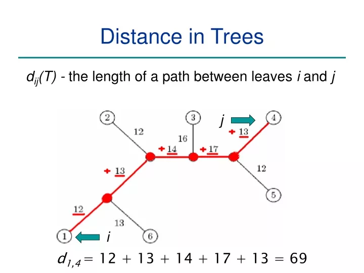
1. j i Distance in Trees dij(T) - the length of a path between leaves i and j d1,4 = 12 + 13 + 14 + 17 + 13 = 69

2. Phylogenetic Tree Reconstruction • Input: • Distance matrix D • Output: • Binary Tree T such that dij(T) = Dij

3. Tree reconstruction for any 3x3 matrix is straightforward We have 3 leaves i, j, k and a center vertex c Reconstructing a 3 Leaved Tree Observe: dic + djc = Dij dic + dkc = Dik djc + dkc = Djk

4. Reconstructing a 3 Leaved Tree(cont’d) dic + djc = Dij + dic + dkc = Dik 2dic + djc + dkc = Dij + Dik 2dic + Djk = Dij + Dik dic = (Dij + Dik – Djk)/2 Similarly, djc = (Dij + Djk – Dik)/2 dkc = (Dki + Dkj – Dij)/2

5. Trees with > 3 Leaves • An tree with n leaves has 2n-3 edges • This means fitting a given tree to a distance matrix D requires solving a system of “n choose 2” equations with 2n-3 variables • This is not always possible to solve for n > 3

6. The Four Point Condition Compute: 1. Dij + Dkl, 2. Dik + Djl, 3. Dil + Djk 2 3 1 2 and3represent the same number:the length of all edges + the middle edge (it is counted twice) 1represents a smaller number:the length of all edges – the middle edge

7. The Four Point Condition • Four point condition: For i,j,k,l two of the sums Dij + Dkl, Dik + Djl, Dil + Djk are equal and the third sum is smaller • Definition : An n x n matrix D is additive provided there exists a tree T with D(T) = D. (Note: T is unique.) • Theorem: D is additive if and only if the four point condition holds for every quartet 1 ≤ i,j,k,l ≤ n

8. Additive Distance Matrices Matrix D is ADDITIVE if there exists a tree T with dij(T) = Dij NON-ADDITIVE otherwise

9. Reconstructing Additive Distances Given T x T D y z w v If we know T and D, but do not know the length of each edge, we can reconstruct those lengths

10. Reconstructing Additive Distances Given T x T y D z a w dvx + dwx = 2 dax + dvw v dax = ½ (dvx + dwx – dvw) day = ½ (dvy + dwy – dvw) D1 daz = ½ (dvz + dwz – dvw)

11. Reconstructing Additive Distances Given T x T y 5 4 D1 b 3 z 3 a 4 c w 7 6 d(a, c) = 3 d(b, c) = d(a, b) – d(a, c) = 3 d(c, z) = d(a, z) – d(a, c) = 7 d(b, x) = d(a, x) – d(a, b) = 5 d(b, y) = d(a, y) – d(a, b) = 4 d(a, w) = d(z, w) – d(a, z) = 4 d(a, v) = d(z, v) – d(a, z) = 6 Correct!!! v D3 D2

12. Distance Based Phylogeny Problem • Goal: Reconstruct an evolutionary tree from a distance matrix • Input: n x n distance matrix Dij • Output: weighted tree T with n leaves fitting D • If D is additive, this problem has a solution and there is a simple algorithm to solve it

13. Find neighboring leavesi and j with parent k Remove the rows and columns of i and j Add a new row and column corresponding to k, where the distance from k to any other leaf m can be computed as: Using Neighboring Leaves to Construct the Tree Dkm = (Dim + Djm – Dij)/2 Compress i and j into k, iterate algorithm for rest of tree

14. Finding Neighboring Leaves • To find neighboring leaves we simply select a pair of closest leaves.

15. Finding Neighboring Leaves • To find neighboring leaves we simply select a pair of closest leaves. WRONG

16. Finding Neighboring Leaves • Closest leaves aren’t necessarily neighbors • i and j are neighbors, but (dij= 13) > (djk = 12) • Finding a pair of neighboring leaves is • a nontrivial problem!

17. Degenerate Triples • A degenerate triple is a set of three distinct elements 1≤i,j,k≤n where Dij + Djk = Dik • Element j in a degenerate triple i,j,k lies on the evolutionary path from i to k (or is attached to this path by an edge of length 0).

18. Looking for Degenerate Triples • If distance matrix Dhas a degenerate triple i,j,k then j can be “removed” from D thus reducing the size of the problem. • If distance matrix Ddoes not have a degenerate triple i,j,k, one can “create” a degenerative triple in D by shortening all hanging edges (in the tree).

19. Shortening Hanging Edges to Produce Degenerate Triples • Shorten all “hanging” edges (edges that connect leaves) until a degenerate triple is found

20. Finding Degenerate Triples • If there is no degenerate triple, all hanging edges are reduced by the same amount δ, so that all pair-wise distances in the matrix are reduced by 2δ. • Eventually this process collapses one of the leaves (when δ = length of shortest hanging edge), forming a degenerate triple i,j,k and reducing the size of the distance matrix D. • The attachment point for j can be recovered in the reverse transformations by saving Dijfor each collapsed leaf.

21. Reconstructing Trees for Additive Distance Matrices Trim(D, δ) for all 1 ≤ i ≠ j ≤ n Dij = Dij - 2δ

22. AdditivePhylogeny Algorithm • AdditivePhylogeny(D) • ifD is a 2 x 2 matrix • T = tree of a single edge of length D1,2 • return T • ifD is non-degenerate • Compute trimming parameter δ • Trim(D, δ) • Find a triple i, j, k in D such that Dij + Djk = Dik • x = Dij • Remove jth row and jth column from D • T = AdditivePhylogeny(D) • Traceback

23. AdditivePhylogeny (cont’d) Traceback • Add a new vertex v to T at distance x from i to k • Add j back to T by creating an edge (v,j) of length 0 • for every leaf l in T • if distance from l to v in the tree ≠ Dl,j • output “matrix is not additive” • return • Extend all “hanging” edges by length δ • returnT

24. Neighbor Joining Algorithm • In 1987 Naruya Saitou and Masatoshi Nei developed a neighbor joining algorithm for phylogenetic tree reconstruction • Finds a pair of leaves that are close to each other but far from other leaves: implicitly finds a pair of neighboring leaves • Advantages: works well for additive and other non-additive matrices, it does not have the flawed molecular clock assumption

25. Neighbor-Joining • Guaranteed to produce the correct tree if distance is additive • May produce a good tree even when distance is not additive Let C = current clusters. Step 1: Finding neighboring clusters Define: u(C) =1/(|C|-2) C’ 2C D(C, C0 ) u(C) measures separation of C from other clusters Want to minimize D(C1, C2) and maximize u(C1) + u(C2) Magic trick: Choose C1 and C2 that minimize D(C1, C2) - (u(C1) + u(C2) ) Claim: Above ensures that Dij is minimal iffi, j are neighbors Proof: Very technical, please read Durbin et al.! 1 3 0.1 0.1 0.1 0.4 0.4 4 2

26. Algorithm: Neighbor-joining Initialization: For n clusters, one for each leaf node Define T to be the set of leaf nodes, one per sequence Iteration: Pick Ci, Cj s.t. D(Ci, Cj) – (u(C1) + u(C2)) is minimal Merge C1 and C2 into new cluster with |C1| + |C2| elements Add a new vertex C to T and connect to vertices C1 and C2 Assign length 1/2 (D(C1, C2) + (u(C1) - u(C2) ) to edge (C1, C) Assign length 1/2 (D(C1, C2) + (u(C2) - u(C1) ) to edge (C2, C) Remove rows and columns from D corresponding to C1 and C2; Add row and column to D for new cluster C Termination: When only one cluster