Download
1 / 75
750 likes | 895 Vues
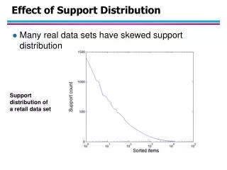
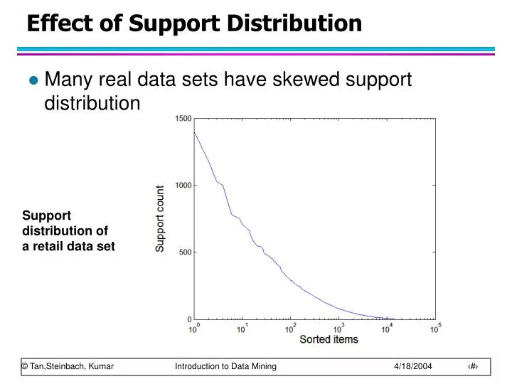
Effect of Support Distribution. Many real data sets have skewed support distribution. Support distribution of a retail data set. Effect of Support Distribution. How to set the appropriate minsup threshold?

E N D
Effect of Support Distribution • Many real data sets have skewed support distribution Support distribution of a retail data set
Effect of Support Distribution • How to set the appropriate minsup threshold? • If minsup is set too high, we could miss itemsets involving interesting rare items (e.g., expensive products) • If minsup is set too low, it is computationally expensive and the number of itemsets is very large • Using a single minimum support threshold may not be effective
Multiple Minimum Support • How to apply multiple minimum supports? • MS(i): minimum support for item i • e.g.: MS(Milk)=5%, MS(Coke) = 3%, MS(Broccoli)=0.1%, MS(Salmon)=0.5% • MS({Milk, Broccoli}) = min (MS(Milk), MS(Broccoli)) = 0.1% • Challenge: Support is no longer anti-monotone • Suppose: Support(Milk, Coke) = 1.5% and Support(Milk, Coke, Broccoli) = 0.5% • {Milk,Coke} is infrequent but {Milk,Coke,Broccoli} is frequent
Multiple Minimum Support (Liu 1999) • Order the items according to their minimum support (in ascending order) • e.g.: MS(Milk)=5%, MS(Coke) = 3%, MS(Broccoli)=0.1%, MS(Salmon)=0.5% • Ordering: Broccoli, Salmon, Coke, Milk • Need to modify Apriori such that: • L1 : set of frequent items • F1 : set of items whose support is MS(1) where MS(1) is mini( MS(i) ) • C2 : candidate itemsets of size 2 is generated from F1instead of L1
Multiple Minimum Support (Liu 1999) • Modifications to Apriori: • In traditional Apriori, • A candidate (k+1)-itemset is generated by merging two frequent itemsets of size k • The candidate is pruned if it contains any infrequent subsets of size k • Pruning step has to be modified: • Prune only if subset contains the first item • e.g.: Candidate={Broccoli, Coke, Milk} (ordered according to minimum support) • {Broccoli, Coke} and {Broccoli, Milk} are frequent but {Coke, Milk} is infrequent • Candidate is not pruned because {Coke,Milk} does not contain the first item, i.e., Broccoli.
Pattern Evaluation • Association rule algorithms tend to produce too many rules • many of them are uninteresting or redundant • Redundant if {A,B,C} {D} and {A,B} {D} have same support & confidence • Interestingness measures can be used to prune/rank the derived patterns • In the original formulation of association rules, support & confidence are the only measures used
Interestingness Measures Application of Interestingness Measure
f11: support of X and Yf10: support of X and Yf01: support of X and Yf00: support of X and Y Computing Interestingness Measure • Given a rule X Y, information needed to compute rule interestingness can be obtained from a contingency table Contingency table for X Y Used to define various measures • support, confidence, lift, Gini, J-measure, etc.
Association Rule: Tea Coffee • Confidence= P(Coffee|Tea) = 0.75 • but P(Coffee) = 0.9 • Although confidence is high, rule is misleading • P(Coffee|Tea) = 0.9375 Drawback of Confidence
Statistical Independence • Population of 1000 students • 600 students know how to swim (S) • 700 students know how to bike (B) • 420 students know how to swim and bike (S,B) • P(SB) = 420/1000 = 0.42 • P(S) P(B) = 0.6 0.7 = 0.42 • P(SB) = P(S) P(B) => Statistical independence • P(SB) > P(S) P(B) => Positively correlated • P(SB) < P(S) P(B) => Negatively correlated
Statistical-based Measures • Measures that take into account statistical dependence
Example: Lift/Interest • Association Rule: Tea Coffee • Confidence= P(Coffee|Tea) = 0.75 • but P(Coffee) = 0.9 • Lift = 0.75/0.9= 0.8333 (< 1, therefore is negatively associated)
Drawback of Lift & Interest Statistical independence: If P(X,Y)=P(X)P(Y) => Lift = 1
There are lots of measures proposed in the literature Some measures are good for certain applications, but not for others What criteria should we use to determine whether a measure is good or bad? What about Apriori-style support based pruning? How does it affect these measures?
Properties of A Good Measure • Piatetsky-Shapiro: 3 properties a good measure M must satisfy: • M(A,B) = 0 if A and B are statistically independent • M(A,B) increase monotonically with P(A,B) when P(A) and P(B) remain unchanged • M(A,B) decreases monotonically with P(A) [or P(B)] when P(A,B) and P(B) [or P(A)] remain unchanged
Comparing Different Measures 10 examples of contingency tables: Rankings of contingency tables using various measures:
Property under Variable Permutation Does M(A,B) = M(B,A)? Symmetric measures: • support, lift, collective strength, cosine, Jaccard, etc Asymmetric measures: • confidence, conviction, Laplace, J-measure, etc
Property under Row/Column Scaling Grade-Gender Example (Mosteller, 1968): 2x 10x Mosteller: Underlying association should be independent of the relative number of male and female students in the samples
Property under Inversion Operation Transaction 1 . . . . . Transaction N
Example: -Coefficient • -coefficient is analogous to correlation coefficient for continuous variables Coefficient is the same for both tables
Property under Null Addition Invariant measures: • support, cosine, Jaccard, etc Non-invariant measures: • correlation, Gini, mutual information, odds ratio, etc
Subjective Interestingness Measure • Objective measure: • Rank patterns based on statistics computed from data • e.g., 21 measures of association (support, confidence, Laplace, Gini, mutual information, Jaccard, etc). • Subjective measure: • Rank patterns according to user’s interpretation • A pattern is subjectively interesting if it contradicts the expectation of a user (Silberschatz & Tuzhilin) • A pattern is subjectively interesting if it is actionable (Silberschatz & Tuzhilin)
Interestingness via Unexpectedness • Need to model expectation of users (domain knowledge) • Need to combine expectation of users with evidence from data (i.e., extracted patterns) + Pattern expected to be frequent - Pattern expected to be infrequent Pattern found to be frequent Pattern found to be infrequent - + Expected Patterns - + Unexpected Patterns
Interestingness via Unexpectedness • Web Data (Cooley et al 2001) • Domain knowledge in the form of site structure • Given an itemset F = {X1, X2, …, Xk} (Xi : Web pages) • L: number of links connecting the pages • lfactor = L / (k k-1) • cfactor = 1 (if graph is connected), 0 (disconnected graph) • Structure evidence = cfactor lfactor • Usage evidence • Use Dempster-Shafer theory to combine domain knowledge and evidence from data
Other issues • Categorical • Continuous • Multi-level
Continuous and Categorical Attributes How to apply association analysis formulation to non-asymmetric binary variables? Example of Association Rule: {Number of Pages [5,10) (Browser=Mozilla)} {Buy = No}
Handling Categorical Attributes • Transform categorical attribute into asymmetric binary variables • Introduce a new “item” for each distinct attribute-value pair • Example: replace Browser Type attribute with • Browser Type = Internet Explorer • Browser Type = Mozilla • Browser Type = Mozilla
Handling Categorical Attributes • Potential Issues • What if attribute has many possible values • Example: attribute country has more than 200 possible values • Many of the attribute values may have very low support • Potential solution: Aggregate the low-support attribute values • What if distribution of attribute values is highly skewed • Example: 95% of the visitors have Buy = No • Most of the items will be associated with (Buy=No) item • Potential solution: drop the highly frequent items
Handling Continuous Attributes • Different kinds of rules: • Age[21,35) Salary[70k,120k) Buy • Salary[70k,120k) Buy Age: =28, =4 • Different methods: • Discretization-based • Statistics-based • Non-discretization based • minApriori
Handling Continuous Attributes • Use discretization • Unsupervised: • Equal-width binning • Equal-depth binning • Clustering • Supervised: Attribute values, v bin3 bin1 bin2
Discretization Issues • Size of the discretized intervals affect support & confidence • If intervals too small • may not have enough support • If intervals too large • may not have enough confidence • Potential solution: use all possible intervals {Refund = No, (Income = $51,250)} {Cheat = No} {Refund = No, (60K Income 80K)} {Cheat = No} {Refund = No, (0K Income 1B)} {Cheat = No}
Discretization Issues • Execution time • If intervals contain n values, there are on average O(n2) possible ranges • Too many rules {Refund = No, (Income = $51,250)} {Cheat = No} {Refund = No, (51K Income 52K)} {Cheat = No} {Refund = No, (50K Income 60K)} {Cheat = No}
Approach by Srikant & Agrawal • Preprocess the data • Discretize attribute using equi-depth partitioning • Use partial completeness measure to determine number of partitions • Merge adjacent intervals as long as support is less than max-support • Apply existing association rule mining algorithms • Determine interesting rules in the output
Approach by Srikant & Agrawal • Discretization will lose information • Use partial completeness measure to determine how much information is lost C: frequent itemsets obtained by considering all ranges of attribute values P: frequent itemsets obtained by considering all ranges over the partitions P is K-complete w.r.t C if P C,and X C, X’ P such that: 1. X’ is a generalization of X and support (X’) K support(X) (K 1) 2. Y X, Y’ X’ such that support (Y’) K support(Y) Given K (partial completeness level), can determine number of intervals (N) Approximated X X
Interestingness Measure {Refund = No, (Income = $51,250)} {Cheat = No} {Refund = No, (51K Income 52K)} {Cheat = No} {Refund = No, (50K Income 60K)} {Cheat = No} • Given an itemset: Z = {z1, z2, …, zk} and its generalization Z’ = {z1’, z2’, …, zk’} P(Z): support of Z EZ’(Z): expected support of Z based on Z’ • Z is R-interesting w.r.t. Z’ if P(Z) R EZ’(Z)
Interestingness Measure • For S: X Y, and its generalization S’: X’ Y’ P(Y|X): confidence of X Y P(Y’|X’): confidence of X’ Y’ ES’(Y|X): expected support of Z based on Z’ • Rule S is R-interesting w.r.t its ancestor rule S’ if • Support, P(S) R ES’(S) or • Confidence, P(Y|X) R ES’(Y|X)
Statistics-based Methods • Example: Browser=Mozilla Buy=Yes Age: =23 • Rule consequent consists of a continuous variable, characterized by their statistics • mean, median, standard deviation, etc. • Approach: • Withhold the target variable from the rest of the data • Apply existing frequent itemset generation on the rest of the data • For each frequent itemset, compute the descriptive statistics for the corresponding target variable • Frequent itemset becomes a rule by introducing the target variable as rule consequent • Apply statistical test to determine interestingness of the rule
Statistics-based Methods • How to determine whether an association rule interesting? • Compare the statistics for segment of population covered by the rule vs segment of population not covered by the rule: A B: versus A B: ’ • Statistical hypothesis testing: • Null hypothesis: H0: ’ = + • Alternative hypothesis: H1: ’ > + • Z has zero mean and variance 1 under null hypothesis
Statistics-based Methods • Example: r: Browser=Mozilla Buy=Yes Age: =23 • Rule is interesting if difference between and ’ is greater than 5 years (i.e., = 5) • For r, suppose n1 = 50, s1 = 3.5 • For r’ (complement): n2 = 250, s2 = 6.5 • For 1-sided test at 95% confidence level, critical Z-value for rejecting null hypothesis is 1.64. • Since Z is greater than 1.64, r is an interesting rule
Min-Apriori (Han et al) Document-term matrix: Example: W1 and W2 tends to appear together in the same document
Min-Apriori • Data contains only continuous attributes of the same “type” • e.g., frequency of words in a document • Potential solution: • Convert into 0/1 matrix and then apply existing algorithms • lose word frequency information • Discretization does not apply as users want association among words not ranges of words
Min-Apriori • How to determine the support of a word? • If we simply sum up its frequency, support count will be greater than total number of documents! • Normalize the word vectors – e.g., using L1 norm • Each word has a support equals to 1.0 Normalize
Min-Apriori • New definition of support: Example: Sup(W1,W2,W3) = 0 + 0 + 0 + 0 + 0.17 = 0.17
Anti-monotone property of Support Example: Sup(W1) = 0.4 + 0 + 0.4 + 0 + 0.2 = 1 Sup(W1, W2) = 0.33 + 0 + 0.4 + 0 + 0.17 = 0.9 Sup(W1, W2, W3) = 0 + 0 + 0 + 0 + 0.17 = 0.17
Multi-level Association Rules • Why should we incorporate concept hierarchy? • Rules at lower levels may not have enough support to appear in any frequent itemsets • Rules at lower levels of the hierarchy are overly specific • e.g., skim milk white bread, 2% milk wheat bread, skim milk wheat bread, etc.are indicative of association between milk and bread
Multi-level Association Rules • How do support and confidence vary as we traverse the concept hierarchy? • If X is the parent item for both X1 and X2, then (X) >= (X1) + (X2) • If (X1 Y1) ≥ minsup, and X is parent of X1, Y is parent of Y1 then (X Y1) ≥ minsup, (X1 Y) ≥ minsup (X Y) ≥ minsup • If conf(X1 Y1) ≥ minconf,then conf(X1 Y) ≥ minconf