Download
1 / 40
400 likes | 640 Vues
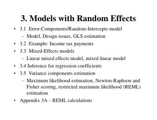
3. Models with Random Effects. 3.1 Error-Components/Random-Intercepts model Model, Design issues, GLS estimation 3.2 Example: Income tax payments 3.3 Mixed-Effects models Linear mixed effects model, mixed linear model 3.4 Inference for regression coefficients

E N D
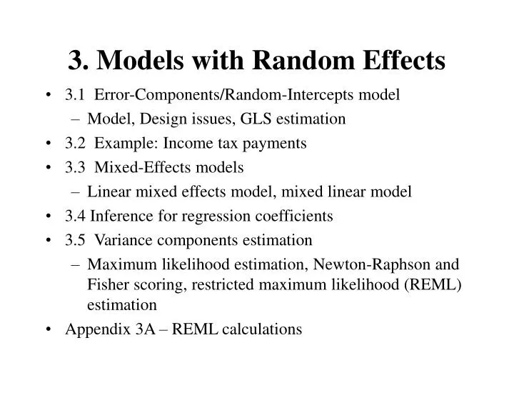
3. Models with Random Effects • 3.1 Error-Components/Random-Intercepts model • Model, Design issues, GLS estimation • 3.2 Example: Income tax payments • 3.3 Mixed-Effects models • Linear mixed effects model, mixed linear model • 3.4 Inference for regression coefficients • 3.5 Variance components estimation • Maximum likelihood estimation, Newton-Raphson and Fisher scoring, restricted maximum likelihood (REML) estimation • Appendix 3A – REML calculations
3.1 Error components model • Sampling - Subjects may consist of a random subset from a population, not fixed subjects • Inference - In the fixed effects models, our inference deals, in part, with subject-specific parameters {ai}. • These parameters are based on the subjects in our sample. • We may wish to make statements about the entire population. • In the fixed effects model, because n is typically large, there are many nuisance parameters {ai}.
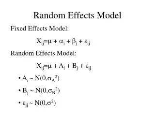
Basic model • The error components model is yit = i + xit´ + it. • This portion of the notation is the same as the basic fixed model. However, now the quantities i are assumed to be random variables, not fixed unknown parameters. • We assume that i are independently and identically distributed (i.i.d) with mean zeroand variance . • We assume that {i } are independent of the error random variables, {it } . • We still assume that xit is a vector of covariates, or explanatory variables, and that is a vector of fixed, yet unknown, population parameters. • In the error components model, we assume no serial correlation, that is, Var i = Ii . • Thus, the variance of the ith subject is Var yi = aJi + Ii = Vi
Traditional ANOVA set-up • Without the covariates, this is the traditional random effects (one way) ANOVA set-up. • This model can be interpreted as arising from a stratified sampling scheme. • We draw a sample from a population of subjects. • We observe each subject over time. • Is there heterogeneity among subjects? One response is to test the null hypothesis H0: sa2 = 0. • Estimates of sa2 are of interest but require scaling to interpret. A more useful quantity to report is sa2 /(sa2 +s 2 ), the intra-class correlation.
Sampling • The experimental design specifies how the subjects are selected and may dictate the model choice. • Selecting subjects based on a (stratified) random sample implies use of the random effects model. • This sampling scheme also suggests that the covariates are random variables. • Selecting subjects based on characteristics suggests using a fixed effects model. • In the extreme, each i represents a characteristic. • Another example is where we sample the entire population. For example, the 50 states in the US.
Error Components Model Assumptions • E (yit |i ) = i + xit β. • {xit,1, ... , xit,K} are nonstochastic variables. • Var (yit |i ) = σ2. • { yit } are independent random variables, conditional on {α1, …, αn}. • yit is normally distributed, conditional on {α1, …, αn}. • E i = 0, Var i = σα2 and {α1, …, αn} are mutually independent. • {αi} is normally distributed.
Observables Representation of the Error Components Model • E yit = xit β. • {xit,1, ... , xit,K} are nonstochastic variables. • Var yit = σ2 + σα2 and Cov (yir, yis) = σα2, for r s. • {yi } are independent random vectors. • { yi } are normally distributed.
Structural Models • What is the population? • A standard defense for a probabilistic approach to economics is that although there may be a finite number of economic entities, there is an infinite range of economic decisions. • According to Haavelmo (1944) • “ … the class of populations we are dealing with does not consist of an infinity of different individuals, it consists of an infinity of possible decisions which might be taken with respect to the value of y.” • See Nerlove and Balestra’s chapter in a monograph edited by Mátyás and Sevestre (1996, Chapter 1) in the context of panel data modeling.
Inference • If you would like to make statements about a population larger than the sample, design the sample to use the random effects model. • If you are simply interested in controlling for subject-specific effects (treating them as nuisance parameters), then use the fixed model. • In addition to sampling and inference, the model design may also be influenced by a desire to increase the degrees of freedom available for parameter estimation. • Degrees of freedom • There are n+K linear regression parameters plus 1 variance parameter in the fixed effects model, compared to only 1+K regression plus 2 variance parameters in the random effects model. • Choose the random effects models to increase the degrees of freedom available for parameter estimation.
Time-constant variables • If the primary interest is in testing for the effects of time-constant variables, then, other things being equal, design the sample to use a random effects model. • An important example of a time-constant variable is a variable that classifies subjects by groups: • Often, we wish to compare the performance of different groups, for example, a “treatment group” and a “control group.” • In the fixed effects model, time-constant variables are perfectly collinear with subject-specific intercepts and hence are inestimable.
GLS estimation • Expressing the model in matrix form, we have E yi = Xib and Var yi = Vi =sa2Ji + s 2Ii. • Ji is a Ti×Ti matrix of ones, Iiis a Ti×Ti identity matrix. • Here, Xiis a Ti×K matrix of explanatory variables, Xi= (xi1, xi2, ... , xiTi) ´. • The generalized least squares (GLS) equations are: • This yields the error-components estimator of b • The variance of the error components estimator is:
Feasible generalized least squares • This assumes that the variance parameters sa2 and s 2 are known . One way to get a “feasible” generalized least squares estimate is: • First run a regression assuming Vi =Ii, ordinary least squares. • Use the residuals to determine estimates of sa2 and s 2 . • This estimation procedure yields estimates of sa2 that can be negative, although unbiased. • Determine bECusing the estimates of sa2 and s 2 . • This procedure could be iterated. However, studies have shown that iterated versions do not improve the performance of the one-step estimators. • There are many ways to estimate the variance parameters: • Regardless of how the estimate is obtained, use it in the GLS estimates. • See Section 3.5 for more details.
Pooling test • Test whether the intercepts take on a common value. That is, do we have to account for subject-specific effects? • Using notation, we wish to test the null hypothesis H0: sa2 = 0. • This is an extension of a Lagrange multiplier statistic due to Breusch and Pagan (1980). • This can be done using the following procedure: • Run the model yit= xit´b + eitto get residuals eit . • For each subject, compute an estimator of sa2 • Compute the test statistic, • Reject H0 if TS exceeds a quantile from an c2 (chi-square) distribution with one degree of freedom.
3.3 Mixed models • The linear mixed-effects model is yit = zit´i + xit´ + it. • This is short-hand notation for the model yit = i1 zit1 + ... + iq zitq +1xit1+... + KxitK+ it • The matrix form of this model is yi= Zii + Xi + i • The responses between subjects are independent, yet we allow for temporal correlation through Var i = Ri. • Further, we now assume that the subject-specific effects {i} are random with mean zero and variance-covariance matrix D. • We assume E i = 0 and Var i = D , a qq (positive definite) matrix. • Subject-specific effects and the noise term are assumed to be uncorrelated, that is, Cov (i , i´) = 0. • Thus, the variance of each subject can be expressed as Var yi = ZiDZi´ + Ri = Vi().
Observables Representation of the Linear Mixed Effects Model • E yi = Xiβ. • {xit,1, ... , xit,K} and {zit,1, ... , zit,q} are nonstochastic variables. • Var yi = ZiDZi + Ri = Vi(τ) = Vi. • {yi} are independent random vectors. • { yi} are normally distributed.
Repeated measures design • This is a special case of the linear mixed effects model. • Here we have i=1, ..., n subjects. A response for each subject is measured based on each of T treatments. The order of treatments is randomized. The mathematical model is: • The main research question of interest is H0: b1 = b2 = ... = bT, no treatment differences. • Here, the order of treatments is randomized and no serial correlation is assumed.
Random coefficients model • Here is another important special case of the panel data mixed model. • Take zit = xit . In this case the panel data mixed model reduces to a random coefficients model, of the form yit= xit´(ai + b) + eit= xit´bi + eit , • where {bi} are random variables with mean b, independent of {eit}. • Two-stage interpretation • 1. Sample subject to get bi • 2. Sample observations with E(yi | bi ) = Xibi and Var(yi | bi ) = Ri. • This yields E yi = Xib and Var yi = XiDXi´ + Ri = Vi.
Variations • Take columns of Zi to be a strict subset of the columns of Xi. • Thus, certain components of biassociated with Zi are stochastic whereas the remaining components that are associated with Xi but not Zi are nonstochastic. • Two-stage interpretation • Use variables Bi such that E bi= Bib. • Then, we have, E yi = XiBib and Var yi = Ri + XiD Xi¢. • This is the random effects model replacing Xi by XiBi and Zi by Xi
More special cases • Inclusion of group effects. Take q = 1 and zit =1 and consider: yit = ai + dg + xgit´b + egit , • for g = 1, ..., G groups, i=1, ..., ng subjects in each group and t=1, ..., Tgi observations of each subject. • Here, {ai} represent random, subject-specific effects and {dg} represent fixed differences among groups. • This model is not estimable when {ai} are fixed effects. • Time-constant variables. We may split the explanatory variables associated with the population parameters into those that vary by time and those that do not (time-invariant). Thus, we can write our panel data mixed model as yit = zit´ ai + x1i´b1 + x2it´b2 + eit • This model is a generalization of the group effects model. • This model is not estimable when {ai} are fixed effects. • Sec Chapter 5 on multilevel models
Mixed Linear Models • Not all models of interest fit into the linear mixed effects model framework, so it is of interest to introduce a generalization, the mixed linear model. • This model is given by y = Z + X + . • Here, for the mean structure, we assume E (y | )= Z + X and E = 0, so that E y = X . • For the covariance structure, we assume • Var = R, Var = D and Cov ( , ´) = 0. • This yields Var y = Z D Z´ + R = V. • This model does not require independence between subjects. • Much of the estimation can be accomplished directly in terms of this more general model. However, the linear mixed effects model provides a more intuitive platform for examining longitudinal data.
Mixed linear model: Special cases • Linear mixed effects model • Take y = (y1´,..., yn´) ´, e = (e1´,..., en´)´, a = (a1´, ..., an´)´, X = (X1´,..., Xn´)´ and Z = block diagonal (Z1,..., Zn) . • With these choices, the model y = Z + X + is equivalent to the model yi= Zii + Xi + i • The two-way error components model is an important panel data model that is not a specific type of linear mixed effects model although it is a special case of the mixed linear model. • This model can be expressed as yit = ai + t + xit´b + eit • This is similar to the error components model but we have added a random time component, t .
3.4 Regression coefficient inference • The GLS estimator of b takes the same form as in the error components model with a more general variance covariance matrix V. • The GLS estimator of bis • Recall Vi = Vi() = ZiDZi´+Ri. • The variance is: • Interpret bGLSas a weighted average of subject-specific gls estimators. bi,GLS is the least squares estimator based solely on the ith subject bi,GLS = (Xi¢Vi-1Xi )-1Xi¢Vi-1yi , Wi,GLS = Xi¢Vi-1Xi
Matrix inversion formula • To simplify the calculations, here is a formula for inverting Vi(t). This matrix has dimension Ti×Ti . Vi(t)-1 = (Ri + ZiDZi´ )-1 = Ri-1 - Ri-1 Zi (D-1 + Zi´Ri-1Zi )-1 Zi´Ri-1 • This is easier to compute if • the temporal covariance matrix Ri has an easily computable inverse and • the dimension q is smaller than Ti . Because the matrix (D-1 + Zi´Ri-1Zi )-1 is only a q×q matrix, it is easier to invert than Vi(t) , aTi×Ti matrix. • For the error components model, this is:
Maximum likelihood estimation • The log-likelihood of a single subject is • Thus, the log-likelihood for the entire data set is L(b, t ) = Sili(b, t ) . • The values of b, t that maximize L(b, t) are the maximum likelihood estimators. • The “score” vector is the vector of derivatives with respect to the parameters. • For notation, let the vector of parameters be q = (b´, t´)´. • With this notation, the score vector is . • If this score has a root, then the root is the maximum likelihood estimator.
Computing the score vector • To compute the score vector, we first take derivatives with respect to b and find the root. That is, • This yields • That is, for fixed covariance parameters t, the maximum likelihood estimators and the generalized least squares estimators are the same.
Robust estimation of standard errors • An alternative, weighted least squares estimator, is • where the weighting matrix Wi,RE depends on the application at hand. If Wi,RE = Vi-1, then bW = bGLS. • Basic calculations show that it has variance • Thus, a robust estimator of the standard error is:
Testing hypotheses • The interest may be in testing H0: βj = βj,0, where the specified value βj,0 is often (although not always) equal to 0. • Use: • Two variants: • One can replace se(bj,GLS) by se(bj,W) to get so-called “robust t-statistics.” • One can replace the standard normal distribution with a t-distribution with the “appropriate” number of degrees of freedom • SAS default is the “containment method.” • We typically will have large number of observations and will be more concerned with potential heteroscedasticity and serial correlation and thus will use robust t-statistics.
Likelihood ratio test procedure • Using the unconstrained model, calculate maximum likelihood estimates and the corresponding likelihood, denoted as LMLE. • For the model constrained using H0: C β = d , calculate maximum likelihood estimates and the corresponding likelihood, denoted as LReduced. • Compute the likelihood ratio test statistic, LRT = 2 (LMLE - LReduced). • Reject H0 if LRT exceeds a percentile from a c2 (chi-square) distribution with p degrees of freedom. The percentile is one minus the significance level of the test. • See Appendix C.7 for more details on the likelihood ratio test.
3.5 Variance component estimation • Maximum Likelihood • Iterative estimation:Newton-Raphson and Fisher Scoring • Restricted maximum likelihood (REML) • Starting values: • Swamy’s method • Rao’s MIVQUE estimators
Maximum likelihood estimation • The concentrated log-likelihood is • Here, the error sum of squares is • In some cases, one can obtain closed forms solutions. • In general, this must be maximized iteratively.
Variance components estimation • Thus, we now maximize the log-likelihood as a function of t only. Then we calculate bMLE(t) in terms of t. • This can be done using either the Newton-Raphson or the Fisher scoring method. • Newton-Raphson. Let L = L(bMLE(t) , t ) , and use the iterative method: • Here, the matrix • is called the “sample information matrix.” • Scoring. Define the expected information matrix H(t) = E ( ) and use
Motivation for REML • Maximum likelihood often produces biased estimator of variance components. • To illustrate, consider the basic cross-sectional regression model: • Let yi = xi´ b + ei, i=1, ..., N, where b is a p 1 vector, {ei} are i.i.d. N(0, s2). • The mle of s2 is (Error SS)/ N, where Error SS is the error sum of squares from the model fit. • This estimate has expectation s2 (N /(N -p)) and thus is a biased estimate of s2.
Further motivation for REML • As another example, consider our basic fixed effects panel data model: • yit = ai + xi´ b + eit, where b is a K 1 vector, {eit} are i.i.d. N(0, s2). • As above, the mle of s2 is (Error SS)/N, where Error SS is the error sum of squares from the model fit. • This estimator has expectation s2 (N-(n+K))/ N and thus is a biased estimate of s2. • The bias is not asymptotically negligible. To illustrate, in the balanced design case, we have N=nT and • bias = s2(nT-(n+K))/ (nT) - s2 = - s2 (n+K)/(nT) @ - s2 /T, for large n.
REML • The acronym REML stands for restricted maximum likelihood. • The idea is to consider only linear combinations of responses {y} that do not depend on the mean parameters. • To illustrate, consider the following generic situation: • the responses are denoted by the vector y, are normally distribution and have mean E y = X b and variance-covariance matrix Var y = V(t). • The dimension of y is N 1 and the dimension of X is Np . • Suppose that we wish to estimate the parameters of the variance component, t .
REML estimation • Define the projection matrix Q = I - X (X´ X)-1 X´. • If X has dimension Np, then the projection matrix Q has dimension NN. • Consider the linear combination of responses Q y. • Some straightforward calculation show that this has mean 0 and variance-covariance matrix Var y = Q V Q. • Because (i) Q y is normally distributed and (ii) the mean and variance do not depend on b , this means that the entire distribution of Q y does not depend on b. • We could also use any linear transform of Q, such as A Q . • That is, the distribution of A Q y is also normally distributed with with a mean and variance that does not depend on b.
Modified likelihood • These observations led Patterson and Thompson (1971) and Harville (1974) to modify our likelihood calculations by considering the “restricted” maximum log-likelihood : • a function of t. • Here, the error sum of squares is • For comparison, the usual log-likelihood is : • The only difference is the term ln det(X´ V(t) X ) ; thus, methods of maximization are the same (that is, using Newton-Raphson or scoring).
Properties of REML estimates • For the case V = s2I, then the REML estimate yields the unbiased estimate of s2. • When p, the number of regressors is small, the MLE and REML estimates of variance components are similar. • When p, the number of regressors is large, REML estimates tend to outperform MLE estimates. • The additional term for the longitudinal data mixed model is
Starting Values • Both Swamy and Rao’s procedures provide useful, non-recursive, variance components estimates • Rao’s MIVQUE estimators are available for a larger class of models (handling serial correlation, for example) • A version of MIVQUE is the default option in SAS PROC MIXED for starting values.
REML versus MLE • Both are likelihood based estimators • They applied to a wide variety of models • They rely on a parametric specification • For likelihood ratio tests, one should not use REML. • Use instead maximum likelihood estimators • Appendix 3A.3 demonstrates the potentially disastrous consequences of using REML estimators for likelihood ratio tests.