Download
1 / 76
1.28k likes | 1.83k Vues
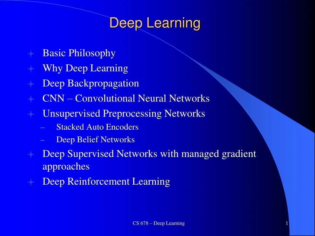
Deep Learning. Basic Philosophy Why Deep Learning Deep Backpropagation CNN – Convolutional Neural Networks Unsupervised Preprocessing Networks Stacked Auto Encoders Deep Belief Networks Deep Supervised Networks with managed gradient approaches Deep Reinforcement Learning.

E N D
Deep Learning • Basic Philosophy • Why Deep Learning • Deep Backpropagation • CNN – Convolutional Neural Networks • Unsupervised Preprocessing Networks • Stacked Auto Encoders • Deep Belief Networks • Deep Supervised Networks with managed gradient approaches • Deep Reinforcement Learning CS 678 – Deep Learning
Deep Learning Overview • Train networks with many layers (vs. shallow nets with just a couple of layers) • Multiple layers work to build an improved feature space • First layer learns 1st order features (e.g. edges…) • 2nd layer learns higher order features (combinations of first layer features, combinations of edges, etc.) • Some models learn in an unsupervised mode and discover general features of the input space – serving multiple tasks related to the unsupervised instances (image recognition, etc.) • Final layer of transformed features are fed into supervised layer(s) • And entire network is often subsequently tuned using supervised training of the entire net, using the initial weightings learned in the unsupervised phase CS 678 – Deep Learning
Deep Net Feature Transformation Supervised Learning ML Model New Feature Space Supervised or unsupervised Learning Original Features CS 678 – Deep Learning
Deep Learning Tasks • For some approaches (CNN, Unsupervised) best when input space is locally structured – spatial or temporal: images, language, etc. vs arbitrary input features • Images Example: view of a learned vision feature layer (Basis) • Each square in the figure shows the input image that maximally activates one of the 100 units CS 678 – Deep Learning
Why Deep Learning • Biological Plausibility – e.g. Visual Cortex • Hastad proof - Problems which can be represented with a polynomial number of nodes with k layers, may require an exponential number of nodes with k-1 layers (e.g. parity) • Highly varying functions can be efficiently represented with deep architectures • Less weights/parameters to update than a less efficient shallow representation • Sub-features created in deep architecture can potentially be shared between multiple tasks • Type of Transfer/Multi-task learning CS 678 – Deep Learning
Neural Networks Sketch • More than just MLPs, but… • Rumelhart 1986 – great early success • Interest subsides a bit in the late 90’s as other models are introduced – SVMs, Graphical models, etc. – each their turn... • Convolutional Neural Nets –LeCun 1989-> Image, speech, etc. • Deep Belief nets (Hinton) and Stacked auto-encoders (Bengio) – 2006 – Unsupervised pre-training followed by supervised. Good feature extractors. • 2012 -> Initial successes with supervised approaches which overcome vanishing gradient, etc., and are more general applicable. Current explosion, but don’t drop all the other tools in your kit! • Stay the course CS 678 – Deep Learning
Early Work • Fukushima (1980) – Neo-Cognitron • LeCun (1998) – Convolutional Neural Networks (CNN) • Similarities to Neo-Cognitron • Many layered MLP with backpropagation • Tried early but without much success • Very slow • Vanishing gradient • Relatively recent work demonstrated significant accuracy improvements by "patiently" training deeper MLPs with BP using fast machines (GPUs) • More general learning! • Much improved since 2012 with lots of extensions to the basic BP algorithm CS 678 – Deep Learning
Vanishing/Exploding Gradient • Error attenuation, long patient training with GPUs, etc • Recent algorithmic improvements - Rectified Linear Units, • better weight initialization, normalization between layers, residual • deep learning, etc. – 1000’s of layers being effectively trained …. CS 678 – Deep Learning
Unstable Gradient • Early layers of MLP do not get trained well • Vanishing Gradient – error attenuates as it propagates to earlier layers – t - z < 1, f '(net), scaled by small initial weights • Leads to very slow training (especially at early layers) • Exacerbated since top couple layers can usually learn any task "pretty well" and thus the error to earlier layers drops quickly as the top layers "mostly" solve the task– lower layers never get the opportunity to use their capacity to improve results, they just do a random feature map • Need a way for early layers to do effective work • Instability of gradient in deep networks: Vanishing or exploding gradient • Product of many terms, which unless “balanced” just right, is unstable • Either early or late layers stuck while “opposite” layers are learning CS 678 – Deep Learning
Rectified Linear Units • f(x) = Max(0,x) More efficient gradient propagation, derivative is 0 or constant, just fold into learning rate • Helps f '(net) issue, but still left with other unstable gradient issues • More efficient computation: Only comparison, addition and multiplication. • Leaky ReLUf(x) = x if x > 0 else ax, where 0 ≤ a <= 1, so that derivate is not 0 and can do some learning for net < 0 (does not “die”). • Lots of other variations • Sparse activation: For example, in a randomly initialized networks, only about 50% of hidden units are activated (having a non-zero output) • Learning in linear range easier for most learning models CS 678 – Deep Learning
Softmax and Cross-Entropy Sum-squared error (L2) loss gradient seeks the maximum likelihood hypothesis under the assumption that the training data can be modeled by Normally distributed noise added to the target function value. Fine for regression but less natural for classification. For classification problems it is advantageous and increasingly popular to use the softmax activation function, just at the output layer, with the cross-entropy loss function. Softmax (softens) 1 of n targets to mimic a probability vector for each output. Cross entropy seeks to to find the maximum likelihood hypotheses under the assumption that the observed (1 of n) Boolean outputs is a probabilistic function of the input instance. Maximizing likelihood is cast as the equivalent minimizing of the negative log likelihood. With new loss and activation functions, we must recalculate the gradient equation. Gradient/Error on the output is just (t-z), no f'(net)! The exponent of softmax is unraveled by the ln of cross entropy. Helps avoid gradient saturation. Common with deep networks, with ReLU activations for the hidden nodes CS 478 – Backpropagation
Convolutional Neural Networks • Niche networks built specifically for problems with low dimensional (e.g. 2-d) grid-like local structure • Character recognition – where neighboring pixels will have high correlations and local features (edges, corners, etc.), while distant pixels (features) are un-correlated • Natural images have the property of being stationary, meaning that the statistics of one part of the image are the same as any other part • Some biological plausibility from visual cortex • While standard NN nodes take input from all nodes in the previous layer, CNNs enforce that a node receives only a smallset of features which are spatially or temporally close to each other called receptive fields from one layer to the next (e.g. 3x3, 5x5), thus enforcing ability to handle local 2-D structure. • Can find edges, corners, endpoints, etc. • Good for problems with local 2-D structure, but lousy for general learning with abstract features having no prescribed feature ordering or locality CS 678 – Deep Learning
Convolutions • Typical MLPs have a connection from every node in the previous layer, and the net value for a node is the scalar dot product of the inputs and weights (e.g. matrix multiply). Convolutional nets are somewhat different: • Nodes still do a scalar dot product (convolution) from the previous layer, but with only a small portion (receptive field) of the nodes in the previous layer – Sparse representation • Every node has the exact same weight values from the preceding layer – Shared parameters, tied weights, a LOT less unique weight values. Regularization by having same weights looking at more input situations • Each node has it’s shared weight convolution computed on a receptive field slightly shifted, from that of it’s neighbor, in the previous layer – Translation invariance. • Each node’s convolution scalar is then passed through a non-linear activation function (ReLU, tanh, etc.) CS 678 – Deep Learning
Convolution Example CS 678 – Deep Learning
Convolutional Neural Networks C layers are convolutions, S layers pool/sample Often starts with fairly raw features at initial input and lets CNN discover improved feature layer for final supervised learner – eg. MLP/BP CS 678 – Deep Learning
CNN – Translation Invariance • The 2-d planes of nodes (or their outputs) at subsequent layers in a CNN are called feature maps • To deal with translation invariance, each node in a feature map has the same weights (based on the feature it is looking for), and each node connects to a different overlapping receptive field of the previous layer • Thus each feature map searches the full previous layer to see if, where, and how often its feature occurs (precise position less critical) • The output will be high at each node in the map corresponding to a receptive field where the feature occurs • Later layers could concern themselves with higher order combinations of features and rough relative positions • Each calculation of a node’s net value, Σxw+b in the feature map, is called a convolution, based on the similarity to standard convolutions CS 678 – Deep Learning
CNN Structure • Each node (e.g. convolution) is calculated for each receptive field in the previous layer • During training the corresponding weights are always tied to be the same (ala BPTT) • Thus a relatively small number of unique weight parameters to learn, although they are replicated many times in the feature map • Each node output in CNN is f(Σxw + b) (ReLU, tanh etc.) • Multiple feature maps in each layer • Each feature map should learn a different translation invariant feature • Since after first layer, there are always multiple feature maps to connect to the next layer, it is a pre-made human decision as to which previous maps the current convolution map receives inputs from, could connect to all or a subset (S2 in figure below) • Convolution layer causes total number of features to increase CS 678 – Deep Learning
Sub-Sampling (Pooling) • Convolution and sub-sampling layers are interleaved • Sub-sampling (Pooling) allows number of features to be diminished, and to pool information • Pooling replaces the network output at a certain point with a summary statistic of nearby outputs • Max-Pooling common (Just as long as the feature is there, take the max, as exact position is not that critical), also averaging, etc. • Pooling smoothsthe data and reduces spatial resolution and thus naturally decreases importance of exactly where a feature was found, just keeping the rough location – translation invariance • 2x2 pooling would do 4:1 compression, 3x3 9:1, etc. • Convolution usually increases number of feature maps, pooling keeps same number of reduced maps (one-to-one correspondence of convolution map to pooled map) as the previous layer CS 678 – Deep Learning
Pooling Example (Summing or averaging) CS 678 – Deep Learning
Pooling (cont.) • Common layers are convolution, non-linearity, then pool (repeat) • Note that pooling always decreases map volumes (unless pool stride = 1, highly overlapped), making real deep nets more difficult. Pooling is sometimes used only after multiple convolved layers and sometimes not at all. • At later layers pooling can make network invariant to more than just translation – learned invariances CS 678 – Deep Learning
CNN Training • Trained with BP but with weight tying in each feature map • Randomized initial weights through entire network • Just average the weight updates over the tied weights in feature map layers • Convolution layer • Each feature map has one weight for each input and one bias • Thus a feature map with a 5x5 receptive field (filter) would have a total of 26 weights, which are the same coming into each node of the feature map • If a convolution layer had 10 feature maps, then only a total of 260 unique weights to be trained in that layer (much less than an arbitrary deep net layer without sharing) • Sub-Sampling (Pooling) Layer • All elements of receptive field max’d, averaged, summed, etc. Result multiplied by one trainable weight and a bias added, then passed through non-linear function (detector, e.g. ReLU) for each pooling node • If a layer had 10 pooling feature maps, then 20 unique weights to be trained • While all weights are trained, the structure of the CNN is currently usually hand crafted with trial and error. • Number of total layers, number of receptive fields, size of receptive fields, size of sub-sampling (pooling) fields, which fields of the previous layer to connect to • Typically decrease size of feature maps and increase number of feature maps for later layers CS 678 – Deep Learning
CNN Hyperparameters • Structure itself, number of layers, size of filters, number of feature maps in convolution layers, connectivity between layers, activation functions, final supervised layers, etc. • Drop-out often used in final fully connected layers for overfit avoidance – less critical in convolution/pooling layers which already regularize due to weight sharing • Stride – Don’t have to test every location for the feature (i.e. stride = 1), could sample more coarsely • Another option (besides pooling) for down-sampling • As is, the feature map would always decrease in volume which is not always desirable - Zero-padding avoids this and lets us maintain up to the same volume • Would shrink fast for large kernel/filter sizes and would limit the depth (number of layers) in the network • Also allows the different filter sizes to fit arbitrary map widths CS 678 – Deep Learning
Convolution Example CS 678 – Deep Learning
Example – LeNet-5 – MNIST Classification To help it all sink in: How many weights to be trained at each layer? 5x5 2x2 5x5 2x2 Fully Connected
LeCun-5 Example Why 32x32 to start with? Actual characters never bigger than 28x28. Just padding the edges so for example the top corner node of the feature map can have a pad of two up and left for its feature map. Same things happens with 14x14 to 10x10 drop from S2 to C3 S2 and S4 non-overlapping and pool by summing – We include here the 4 unweighted connections C3: 6 maps connect to 3, 9 to 4, and 1to all 6. Forces discovery of more diverse feature combinations. Table 1 only considers contiguous subsets of 3, and more mixed subsets of 4 feature maps, and one with all – early heuristic attempt which is less crucial, could just connect to all or other variations are fine LeCun used a special RBF output approach in his LeCun-5 model. Could commonly have just gone into an output layer at F6 with 10 output nodes. Then would have been 10*(120+1) = 1210 weights going to the last output layer ~340,000 total connections, with 60,000 trainable parameters 97% of which are in the final MLP
ILSVRC Image net Large Scale Vision Recognition Competition RGB: 224 x 224 x 3 = 150,528 raw real valued features CS 678 – Deep Learning
Example CNNs Structures ILSVRC winners • Note Pooling considered part of the layer • 96 convolution kernels, then 256, then 384 • Stride of 4 for first convolution kernel, 1 for the rest • Pooling layers with 3x3 receptive fields and stride of 2 throughout • Finishes with fully connected (fc) MLP with 2 hidden layers and 1000 output nodes for classes CS 678 – Deep Learning
Increasing Depth CS 678 – Deep Learning
CNN Summary • High accuracy for image applications – Breaking all records and doing it using just using just raw pixel features! • Special purpose net – Just for images or problems with strong grid-like local spatial/temporal correlation • Once trained on one problem (e.g. vision) could use same net (often tuned) for a new similar problem – general creator of vision features • Unlike traditional nets, handles variable sized inputs • Same filters and weights, just convolve across different sized image and dynamically scale size of pooling regions (not # of nodes), to normalize • Different sized images, different length speech segments, etc. • Lots of hand crafting and CV tuning to find the right recipe of receptive fields, layer interconnections, etc. • Lots more Hyperparameters than standard nets, and even than other deep networks, since the structures of CNNs are more handcrafted • CNNs getting wider and deeper with speed-up techniques (e.g. GPU, ReLU, etc.) and lots of current research, excitement, and success CS 678 – Deep Learning
Unsupervised Pre-Training • Began the hype of Deep-Learning (2006) • Before CNNs were fully recognized for what they could do • Less popular at the moment, with recent supervised success, but still at the core of many new research directions including generative deep networks • Unsupervised Pre-Training uses unsupervised learning in the deep layers to transform the inputs into features that are easier to learn by a final supervised model • Unsupervised training between layers can decompose the problem into distributed sub-problems (with higher levels of abstraction) to be further decomposed at subsequent layers • Often not a lot of labeled data available while there may be lots of unlabeled data. Unsupervised Pre-Training can take advantage of unlabeled data. Can be a huge issue for some tasks. • Unsupervised and Semi-Supervised • Self-Taught Learning CS 678 – Deep Learning
Self Taught vs Unsupervised Learning • When using Unsupervised Learning as a pre-processor to supervised learning you are typically given examples from the same distribution as the later supervised instances will come from • Assume the distribution comes from a set containing just examples from a defined set up possible output classes, but the label is not available (e.g. images of car vs trains vs motorcycles) • In Self-Taught Learning we do not require that the later supervised instances come from the same distribution • e.g., Do self-taught learning with any images, even though later you will do supervised learning with just cars, trains and motorcycles. • These types of distributions are more readily available than ones which just have the classes of interest (i.e. not labeled as car or train or motorcycle) • However, if distributions are very different… • New tasks share concepts/features from existing data and statistical regularities in the input distribution that many tasks can benefit from • Can re-use well-trained nets as starting points for other tasks • Note similarities to supervised multi-task and transfer learning • Both unsupervised and self-taught approaches reasonable in deep learning models CS 678 – Deep Learning
Greedy Layer-Wise Training • Train first layer using your data without the labels (unsupervised) • Since there are no targets at this level, labels don't help. Could also use the more abundant unlabeled data which is not part of the training set (i.e. unsupervised and/or self-taught learning). • Then freeze the first layer parameters and start training the second layer using the output of the first layer as the unsupervised input to the second layer • Repeat this for as many layers as desired • This builds the set of robust features • Use the outputs of the final layer as inputs to a supervised layer/model and train the last supervised layer(s) (leave early weights frozen) • Unfreeze all weights and fine tune the full network by training with a supervised approach, given the pre-training weight settings CS 678 – Deep Learning
Deep Net with Greedy Layer Wise Training Supervised Learning ML Model New Feature Space Unsupervised Learning Original Inputs CS 678 – Deep Learning
Greedy Layer-Wise Training • Greedy layer-wise training avoids many of the problems of trying to train a deep net in a supervised fashion • Each layer gets full learning focus in its turn since it is the only current "top" layer (no unstable gradient issues, etc.) • Can take advantage of unlabeled data • When you finally tune the entire network with supervised training the network weights have already been adjusted so that you are in a good error basin and just need fine tuning. This helps with problems of • Ineffective early layer learning • Deep network local minima • We will discuss the two early landmark approaches • Deep Belief Networks • Stacked Auto-Encoders CS 678 – Deep Learning
Auto-Encoders • A type of unsupervised learning which discovers generic features of the data • Learn identity function by learning important sub-features • Compression, etc. – Undercomplete|h| < |x| • For |h| ≥ |x| (Overcomplete case more common in deep nets) use regularized autoencoding: Loss function includes regularizer to make sure we don’t just pass through the data (e.g. sparsity, noise robustness, etc.)
Stacked Auto-Encoders Bengio (2007) – After Deep Belief Networks (2006) Stack many (sparse) auto-encoders in succession and train them using greedy layer-wise training Drop the decode output layer each time
Stacked Auto-Encoders Do supervised training (can now only used labeled examples) on the last layer using final features Then do supervised training on the entire network to fine- tune all weights
Sparse Encoders • Auto encoders will often do a dimensionality reduction • PCA-like or non-linear dimensionality reduction • This leads to a "dense" representation which is nice in terms of parsimony • All features typically have non-zero values for any input and the combination of values contains the compressed information • However, this distributed and entangled representation can often make it more difficult for successive layers to pick out the salient features • A sparse representation uses more features where at any given time many/most of the features will have a 0 value • Thus there is an implicit compression each time but with varying nodes • This leads to more localist variable length encodings where a particular node (or small group of nodes) with value 1 signifies the presence of a high-order feature (small set of bases) • A type of simplicity bottleneck (regularizer) • This is easier for subsequent layers to use for learning CS 678 – Deep Learning
Sparse Representation For bases below, which is easier to see intuition for current pattern - if a few of these are on and the rest 0, or if all have some non-zero value? Easier to learn if sparse CS 678 – Deep Learning
How do we implement a sparse Auto-Encoder? • Use more hidden nodes in the encoder • Use regularization techniques which encourage sparseness (e.g. a significant portion of nodes have 0 output for any given input) • Penalty in the learning function for non-zero nodes • Weight decay • etc. • De-noising Auto-Encoder • Stochastically corrupt training instance each time, but still train auto-encoder to decode the uncorrupted instance, forcing it to de-noise and learn conditional dependencies within the instance • Improved empirical results, handles missing values well CS 678 – Deep Learning
Stacked Auto-Encoders • Concatenation approach (i.e. using both hidden features and original features in final (or other) layers) can be better if not doing fine tuning. If fine tuning, the pure replacement approach can work well. • Always fine tune if there is a sufficient amount of labeled data • For real valued inputs, MLP training is like regression and thus could use linear output node activations, still ReLU at hidden • Stacked Auto-Encoders empirically not quite as accurate as DBNs (Deep Belief Networks) • (with De-noising auto-encoders, stacked auto-encoders competitive with DBNs) • Not generative like DBNs, though recent work with de-noising auto-encoders may allow generative capacity CS 678 – Deep Learning
Deep Belief Networks (DBN) • Geoff Hinton (2006) – Beginning of Deep Learning hype – outperformed kernel methods on MNIST – Also generative • Uses Greedy layer-wise training but each layer is an RBM (Restricted Boltzmann Machine) • RBM is a constrained Boltzmann machine with • No lateral connections between hidden (h) and visible (x) nodes • Symmetric weights • Does not use annealing/temperature, but that is all right since each RBM not seeking a global minima, but rather an incremental transformation of the feature space • Typically uses probabilistic logistic node, but other activations possible CS 678 – Deep Learning
RBM Sampling and Training • Initial state typically set to a training example x (can be real valued) • Because of RBM sampling is simple iterative back and forth process • P(hi= 1|x) = sigmoid(Wix + ci) = 1/(1+e-net(hi)) // ci is hidden node bias • P(xi= 1|h) = sigmoid(W'ih + bi) = 1/(1+e-net(xi)) // bi is visible node bias • Contrastive Divergence (CD-k): How much contrast (in the statistical distribution) is there in the divergence from the original training example to the relaxed version after k relaxation steps • Then update weights to decrease the divergence as in Boltzmann • Typically just do CD-1 (Good empirical results) • Since small learning rate, doing many CD-1 updates is similar to doing fewer versions of CD-k with k > 1 • Note CD-1 just needs to get the gradient direction right, which it usually does, and then change weights in that direction according to the learning rate CS 678 – Deep Learning
RBM Update Notes and Variations • Binomial unit means the standard MLP sigmoid unit • Q and P are probability distribution vectors for hidden (h) and visible/input (x) vectors respectively • During relaxation/weight update can alternatively do updates based on the real valued probabilities (sigmoid(net)) rather than the 1/0 sampled logistic states • Always use actual/binary values from initial x -> h • Doing this makes the hidden nodes a sparser bottleneck and is a regularizer helping to avoid overfit • Could use probabilities on the h -> x and/or final x -> h • in CD-k the final update of the hidden nodes usually use the probability value to decrease the final arbitrary sampling variation (sampling noise) • Lateral restrictions of RBM allow this fast sampling CS 678 – Deep Learning
RBM Update Variations and Notes • Initial weights, small random, 0 mean, sd ~ .01 • Don't want hidden node probabilities early on to be close to 0 or 1, else slows learning, since less early randomness/mixing? Note that this is a bit like annealing/temperature in Boltzmann • Set initial x bias values as a function of how often node is on in the training data, and h biases to 0 or negative to encourage sparsity • Better speed when using momentum (~.5) • Weight decay good for smoothing and also encouraging more mixing (hidden nodes more stochastic when they do not have large net magnitudes) • Also a reason to increase k over time in CD-k as mixing decreases as weight magnitudes increase CS 678 – Deep Learning
Deep Belief Network Training • During execution can iterate multiple times at the top RBM layer Same greedy layer-wise approach First train lowest RBM (h0 – h1) using RBM update algorithm (note h0 is x) Freeze weights and train subsequent RBM layers Then connect final outputs to a supervised model and train that model Finally, unfreeze all weights, and fine tune as an MLP using the initial weights found by DBN training Can do execution as just the tuned MLP or as the RBM sampler with the tuned weights CS 678 – Deep Learning
Can use DBN as a Generative model to create sample x vectors • Initialize top layer to an arbitrary vector (commonly a training set vector) • Gibbs sample (relaxation) between the top two layers m times • If we initialize top layer with values obtained from a training example, then need less Gibbs samples • Pass the vector down through the network, sampling with the calculated probabilities at each layer • Last sample at bottom is the generated x vector (can be real valued if we use the probability vector rather than sample) Alternatively, can start with an x at the bottom, relax to a top value, then start from that vector when generating a new x, which is the dotted lines version. More like standard Boltzmann machine processing.