Download
1 / 50
500 likes | 702 Vues
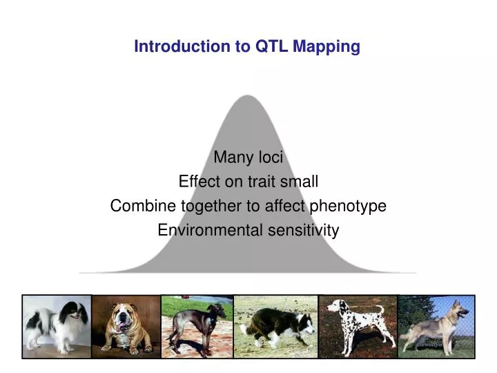
Introduction to QTL Mapping. Many loci. Effect on trait small. Combine together to affect phenotype. Environmental sensitivity. Genetic Architecture of Quantitative Traits. Loci?. Distribution of effects on trait?. Distribution of pleiotropic effects (including fitness).

E N D
Introduction to QTL Mapping Many loci Effect on trait small Combine together to affect phenotype Environmental sensitivity
Genetic Architecture of Quantitative Traits Loci? Distribution of effects on trait? Distribution of pleiotropic effects (including fitness) Distribution of context-dependent effects? Sex Environment Genetic background (epistasis) Causal molecular variant? Allele frequency? QTL Mapping
QTL Mapping • QTL effects too small to be detected by Mendelian segregation • Need to map QTLs by linkage to marker loci with genotypes than can be unambiguously scored • Principle dates back to 1923, but abundant, polymorphic molecular markers only relatively recently available • Most studies use single nucleotide polymorphism (SNP) markers and insertion/deletion (indel) markers • Massively parallel sequencing technology is revolutionizing our ability to rapidly map QTLs
QTL Mapping: A Primer Linkage Mapping Association Mapping Map QTLs in pedigrees or populations derived from crosses of inbred lines Map QTLs in individuals from an outbred population Population sample of individuals with genetic variation for the trait Two (or more) parental strains that differ genetically for trait Molecular markers (whole genome or candidate gene) Molecular markers that distinguish the parental strains Mapping population: Genotype all individuals for markers Measure trait phenotype Mapping population: Genotype all individuals for markers Measure trait phenotype Map QTLs by linkage to markers: Single marker analysis Interval mapping Map QTLs by Linkage Disequilibrium (LD) with markers
Linkage Mapping: Find Parental Strains H2 = 0.58 H2 = 0.56 H2 = 0.23 H2 = 0.54
Linkage Mapping: Create Mapping Population P1 P2 F1 BC1: F1 P1 F2: F1 F1 BC2: F1 P2 RILs
Linkage Mapping: Test for Associations Between Markers and Trait • M1 - - - A1 - - N1- - - - - - - O1 M2 - - - A2 - - N2- - - - - - - O2 • M1 - - - A1 - - N1 - - - - - - -O1 vs. M2 - - - A2 - - N2- - - - - - - O2 • Test for: • Linkage of a QTL (A) to individual markers (M, N, or O) = single marker analysis • QTL in each interval in turn (M-N and N-O) = interval mapping • If there is a difference in trait mean between marker genotype classes, then a QTL is linked to the marker • Infer chromosomal locations and effects (a, d) of QTLs
Line Cross Analysis: Single Markers M Marker locus A QTL c recombination fractionbetween M and A M A c
Line Cross Analysis: Single Markers Generation Genotype Value P1 M1A1/ M1A1a P2 M2A2/ M2A2–a F1 M1A1 / M2A2d F1 gametes: Genotype Frequency M1A1 (1 – c)/2 M2A2 (1 – c)/2 M1A2c/2 M2A1c/2 M A Non-recombinant genotypes c Recombinant genotypes
Line Cross Analysis: Single Markers, F2 Mapping Population • Random mating of the F1 gives 10 possible F2 genotypic • classes. • The contribution of each marker genotype class to the F2 mean • is obtained by multiplying the frequency of each genotype by its • genotypic value, then summing within marker genotype classes. • We want actual means, which are got by dividing the • contribution to the F2 mean by the frequency of that marker class, • which is the Mendelian segregation ratio of ¼ for the homozygotes • and ½ for the heterozygotes.
F2 Genotypes With One Marker Locus, M, and a Linked QTL, A • Genotype Freq. Value Marker Total Contribution Actual • Class Freq. to F2 Mean Mean • M1A1/M1A1 (1 – c)2/4 a • M1A1/M1A2 c(1 – c)/2 d M1/M1 ¼ a(1 – 2c)/4 a(1 – 2c) M1A2/M1A2c 2/4 –a + dc(1 – c)/2 + 2dc(1 – c) • M1A1/M2A1c(1 – c)/2 a • M1A1/M 2A2 (1 – c)2/2 d • M1/M2 ½ d[(1 – c)2 + c2]/2 d[(1 – c)2 +c2] • M1A2/M2A1c2/2 d • M1A2/M2A2c(1 – c)/2 –a • M2A1/M2A1c2/4 a • M2A1/M2A2c(1 – c)/2 dM2/M2 ¼ – a(1 – 2c)/4 – a(1 – 2c) • M2A2/M2A2 (1 – c)2/4 –a + dc(1 – c)/2 +2dc(1 – c)
F2 Genotypes With One Marker Locus, M, and a Linked QTL, A The following two contrasts of marker class means are functions of a and d: Contrast 1: (M1/M1– M2/M2)/2 = a(1 –2c) Contrast 2: M1/M2 – [(M1/M1 + M2/M2)/2] = d(1 –2c)2 This contrast, in combination with the first, therefore allows estimation of d/a, but will always be underestimated by (1 –2c)
F2 Genotypes With One Marker Locus, M, and a Linked QTL, A • In summary: • A significant difference in the mean value of a quantitative • trait between homozygous marker genotype classes indicates • linkage of a QTL and the marker locus. • Estimates of a and d/a from single marker analysis are • confounded with recombination frequency, and will generally • underestimate the true values by (1 –2c). • Example: The true effect is a = 1, d = 0. • Expected estimates for a as a function of c: • c a • 0 1 • 0.1 0.8 • 0.25 0.5 • 0.5 0
Interval Mapping Analysis M A N c1 c2 With complete cross-over interference: c = c1 + c2 (True for c < 0.1 = 10 cM) c
Line Cross Analysis: Interval Mapping Generation Genotype Value P1 M1A1N1/M1A1N1 a P2 M2A2N2/M2A2N2 –a F1 M1A1N1/M2A2N2 d F1 gametes: Genotype Frequency M1A1N1 (1–c)/2 M2A2 N2 (1–c)/2 M1A2N2c1/2 M2A1N1c1/2 M1A1N2c2/2 M2A2N1c2/2 Recombinant genotypes Non-recombinant genotypes • Example: Back-cross (BC) mapping population: • Tabulate BC genotypes, frequencies and means, assuming no double recombination. • Calculate expected marker genotype means.
BC Genotypes With Two Linked Markers, M and N, and a linked QTL, A F1 backcrossed to M1A1N1. Gamete Freq. Value Marker Freq. Contribution to Actual Type Class BC Mean Mean M1A1N1 (1–c)/2 a M1N1/M1N1 (1–c)/2 a(1–c)/2 a M1A1N2c2/2 a M1N1/M1N2c/2 (ac2+dc1)/2 (ac2 + dc1)/c M1A2N2 c1/2 d M2A1N1c1/2 a M1N1/M2N1 c/2 (ac1+dc2)/2 (ac1 + dc2)/c M2A2N1 c2/2 d M2A2N2 (1–c)/2 d M1N1/M2N2 (1–c)/2 d(1–c)/2 d
BC Genotypes With Two Linked Markers, M and N, and a linked QTL, A In a manner similar to the single marker example, contrasts between backcross marker class means (γ and δ below) estimate the effects of the QTL. In contrast to the single marker example, the map position relative to the flanking markers can also be estimated: M1N1/M1N1– M1N1/M2N2 = a– d = γ M1N1/M1N2 – M1N1/M2N1 = (a– d)(c2– c1)/c = δ
BC Genotypes With Two Linked Markers, M and N, and a linked QTL, A The estimate of a is unbiased only if d = 0, so recessive QTLs may not be detected. This problem can be overcome by backcrossing to both parental lines, or by using an F2 design. Note: c is assumed to be known, so c1 and c2 can be estimated: δ/γ = (c2– c1)/c = (c– 2c1)/c and solve for c1.
Association Mapping: Collect Population Phenotypes and Genotypes H2 = 0.58 H2 = 0.56 H2 = 0.23 H2 = 0.54
Association Mapping • Associationmapping utilizes historical recombination in random mating populations to identify QTLs, measured by linkage disequilibrium (LD) • LD is a measure of the correlation in gene frequencies between two loci.
Linkage Disequilibrium (LD) • Consider locus A with alleles A1 and A2 at frequencies p1 and p2 respectively, and locus B with alleles B1 and B2 at frequencies q1 and q2 respectively. • If the gene frequencies at these loci are uncorrelated, the expected frequency of each gamete type is the product of the allele frequencies at each locus separately. • The gamete types are called HAPLOTYPES because we describe the genetic constitution of a haploid gamete. • For two loci there are only 4 gamete types: A1B1, A1B2, A2B1 and A2B2.
Linkage Disequilibrium (LD) Gamete Type Expected Observed (Haplotype) Frequency Frequency A1B1p1q1 = P11 A1B2p1q2 = P12 A2B1p2q1 = P21 A2B2p2q2 = P22 Where p1 + p2 = 1 q1 + q2 = 1 If allele frequencies are uncorrelated, the population is in ‘linkage equilibrium’, and P11P22 - P12P21 = 0
Linkage Disequilibrium (LD) • If allele frequencies are non-randomly associated, the gamete frequencies are not the simple product of the allele frequencies, but depart from this by amount D • D is the coefficient of linkage disequilibrium Gamete Types Expected Frequency Observed (Haplotypes) (Disequilibrium) Frequency A1B1p1q1 + D = P11 A1B2p1q2– D = P12 A2B1p2q1– D = P21 A2B2p2q2 + D = P22 and P11P22– P12P21 = D
Linkage Disequilibrium Linkage Equilibrium A1B1 A1B1 A2B2 A2B2 A1B2 A2B2 A2B2 A1B1 A2B1 A2B2 A2B2 A1B2 A2B2 A2B1 A2B2 A1B1 A1B1 A1B2 A1B1 A1B1 A2B2 A1B2 A1B1 A1B1 A2B1 A1B1 A1B1 A2B2 A1B1 A2B2 A2B1 A2B2 • Numerical value of D depends on gene frequencies at the two loci. • Sign of D is arbitrary for molecular markers; consider absolute value. • Highest value of D for p1 = p2 = q1 = q2 = 0.5, and gamete types A1B2 and A2B1 are missing (complete linkage disequilibrium); D is then 0.25.
Linkage Disequilibrium (LD) Because of the dependence on gene frequency, values of D are typically scaled by the observed gene frequencies. • 1. D'= D/Dmax • Dmaxis the smaller of p1q2 or p2q1. This is because: • P12 = p1q2 – D≥0; D≤ p1q2 • P21= p2q1 – D≥0; D≤ p2q1 • Maximum values of D' is 1. • 2. r2 = D2/p1p2q1q2 • Expected value in equilibrium population is r2 = E(r2) = 1/(1 + 4Nc), where N is the effective population size and c is the recombination fraction between the two loci. • In principle one can use this relationship to estimate c, but r2 has very large statistical and genetic sampling variances, so in practice this relationship is not very useful.
Linkage Disequilibrium (LD) • Causes of LD: • Mutation (a new mutant allele is initially in complete linkage disequilibrium with all other loci in the genome) • Admixture between populations with different gene frequencies • Natural selection for particular combinations of alleles • Population bottlenecks (chance sampling of small number of haplotypes)
Linkage Disequilibrium (LD) c= 0.001 c= 0.005 c= 0.01 c= 0.05 c= 0.1 c= 0.5 • D declines in successive generations in a random mating population by an amount which depends on the recombination fraction, c. • Dt = D0(1 – c)t after t generations of random mating. • With unlinked loci and free recombination (c = 0.5) D is halved by each generation of random mating; with linked loci D decays more slowly.
Linkage Disequilibrium (LD) Disequilibrium between pairs of loci in random mating populations depends on population history, but is expected to be small unless the loci are very tightly linked. Then Now
Association Mapping • Use molecular polymorphism and phenotypic information from samples of alleles from a random mating population to determine whether there is an association with the trait phenotype. • Can be done for candidate gene, QTL region, or whole genome. • Depending on the scale of LD, one can use LD for fine-mapping QTL, and even causal variants. • LD large in populations that have undergone recent bottlenecks in population size, from a founder event or artificial selection • LD small in large, near equilibrium outbred populations (e.g., Drosophila). • CAVEAT: Population admixture can cause false positive associations if marker frequencies and trait values are different between populations
Association Mapping Cases Controls • Quantitative traits: • Group data by genotype for each marker • Assess if there is a difference between the mean of the trait between different alleles of a marker genotype • If so, the locus affecting the trait is in LD with the marker locus Frequency • Categorical traits: • Group data according to whether individuals are affected or not affected • Determine if there is a difference in genotype frequencies or allele frequencies between cases and controls • If so, the locus affecting the trait is in LD with the marker locus Phenotype
Association Mapping • Association mapping underestimates QTL effects unless the molecular marker genotyped is the casual variant • Let be the effect attributable to the causal variant, and a the estimated effect. • = [p(1 – p)/D]a, where p is the frequency of the polymorphic site and D is the LD between the causal QTN and the poylmorphic site associated with it. • D p(1 – p) (maximum p(1 – p) = 0.25), so a
Linkage Mapping: Statistical Considerations • t-tests, ANOVA, marker regressions or more sophisticated maximum likelihood (ML) methods can be used to assess differences in trait phenotype between marker genotypes. • The parental lines will differ at many loci affecting the trait of interest; therefore QTLs unlinked to the markers under consideration will segregate in the F2 or backcross generation. • Methods for dealing with multiple QTL simultaneously (e.g., composite interval mapping) reduce the variance within marker genotype classes and improve estimates of map positions and of effects.
Linkage Mapping: Statistical Considerations • Many markers are tested for linkage to a QTL in a genome scan. • The number of false positives increases with the number of tests. • With n independent tests, the level for each should be set to α/n (a Bonferroni correction). • The number of independent tests will be less than the number of markers because of linked markers. • Permutation tests are typically used to determine appropriate experiment-wise significance levels, accounting for multiple tests and correlated markers. Likelihood ratio
Permutation Test –logP
Linkage Mapping: Power and Sample Size • How large must the experiment be to detect a difference δbetween the two homozygous marker genotypes? • For simplicity, assume the QTL is completely linked to the marker ( c = 0) and that a t-test is used to judge the significance of the difference of two marker class means. • n ≥ 2 (zα + z2β)2/(δ/σP)2 • σP phenotypic standard deviation within marker-classes • α false positive (Type I) error rate (0.05) • β false negative (Type II) error rate (0.1) • z ordinate of the normal distribution corresponding to its subscript • zα = 1.96 andz2β = 1.28
Linkage Mapping: Power and Sample Size F2 BC n = number per marker class N = number of total mapping population For strictly additive effects, FA2 = 2pq*2FP2 • Easy to detect QTLs with large effects • Need large sample sizes to detect QTLs with moderate to small effects • The power to detect a difference in mean between two marker genotypes depends on δ/σP;strategies to reduce σP can increase power (e.g., progeny testing, RI lines).
Linkage Mapping: Recombination and Sample Size Number of marker genotypes needed to localize QTLs per 100 cM Number of individuals needed to detect at least one recombinant in an interval of size c (c = 100cM)
Linkage Mapping: Power, Recombination and Sample Size • Large numbers necessary to detect QTL AND estimate location. • For an F2 design, need 336 individuals to detect QTL with large effect (δ/σP = 0.5) x 59 individuals to ensure the QTL is mapped to a 5 cM region = 19,824 individuals in total and 416,304 marker genotypes per 100 cM. • QTL mapping is in practice an iterative procedure, where QTLs are first mapped to broad genomic regions in a genome scan, followed by high resolution mapping to localize genes within each QTL region. • Genotyping by sequencing is changing this strategy, facilitating rapid, fine mapping of QTLs.
Association Mapping: Power and Sample Size q = 0.1 q = 0.25 q = 0.5 • q = frequency of rare allele • LD mapping has the same power as linkage mapping in an F2 population for intermediate gene frequencies, but much reduced power as the frequency of the rare allele decreases (the number of homozygotes in the population is q2) • This calculation assumes the marker is the causal variant; even larger samples are necessary if the marker is in LD with the causal variant • Easy to detect intermediate frequency variants with large effects • Hard to detect rare variants with small effects
Association Mapping: Recombination and Sample Size c = 0.01 c = 0.005 c = 0.001 • Expected frequency of recombinants after t generations of recombination in a random mating population • Higher frequency of recombinants in random mating population means smaller sample sizes required for high resolution mapping than linkage studies
Association Mapping: Recombination and Sample Size • Number of markers depends on scale and pattern of LD • Small population size = large LD tracts = few markers required for QTL detection, but localization poor (dogs). Favorable situation for whole genome LD scan. • Large population size = small LD tracts =many markers required for QTL detection, but localization precise, maybe to level of QTN (Drosophila). Favorable situation for candidate gene re-sequencing. • LD patterns not constant across genome, but vary with local recombination rate, regions under natural selection • Knowing patterns of LD can guide experimental design
Strategies to Increase Power • Selective genotyping: Measure many individuals (several thousands), but only genotype the extreme tails • Selective genotyping and detect gene frequency differences between tails of distribution by pooling high and low samples (bulk segregant analysis) followed by next generation sequencing of pools
Strategies to Increase Genetic Diversity • Estimates of the number of QTL are minimum estimates: • Experiments are limited in their power to separate closely linked loci • There must always be other loci with effects too small to be detected by an experiment of a particular size • The loci found are those differentiating the two strains compared • Other loci would probably be found in other strains • Can increase genetic diversity by: • Artificial selection for high and low trait values from large heterogeneous base population, then inbreeding to construct parental stocks for mapping • Mapping population derived from crosses of several inbred strains, either RI lines or large outbred population maintained for many generations
High Resolution Mapping • Construction of near-isoallelic lines (NIL) • backcross to one of parental strains • select for markers flanking QTL and against markers flanking other QTL • Fine-scale recombination • backcross NIL to one of parental strains • select for recombinants within NIL interval using additional markers • progeny test recombinant genotypes to map QTL to 2 cM or less. • Deficiency mapping (in Drosophila) • Change strategy from linkage to association mapping
G1 G2 G3 Gt
Effect +a a a a +a +a +a a a a +a +a
QTL End Game: Proving QTL Corresponds to Candidate Gene • Supporting evidence: • Potentially functional DNA polymorphisms • Differences mRNA expression between alleles • Expression of RNA/protein in relevant tissues • Replicated associations in different populations • Quantitative complementation QTL alleles and mutant allele • More concrete evidence: • Create mutants in the candidate gene that affect the trait (transposon tagging) • Transgenic rescue • Demonstrate functional differences between alleles by knocking-in alternate alleles by homologous recombination