Download
1 / 16
180 likes | 467 Vues
Dynamics of a Ratio-Dependent Predator-Prey Model with Nonconstant Harvesting Policies. Catherine Lewis and Benjamin Leard. August 1 st , 2007. Predator-Prey Models.

E N D
Dynamics of a Ratio-Dependent Predator-Prey Model with Nonconstant Harvesting Policies Catherine Lewis and Benjamin Leard August 1st, 2007
Predator-Prey Models • 1925 & 1926: Lotka and Volterra independently propose a pair of differential equations that model the relationship between a single predator and a single prey in a given environment: Variable and Parameter definitions x – prey species population y – predator species population r – Intrinsic rate of prey population Increase a – Predation coefficient b – Reproduction rate per 1 prey eaten c – Predator mortality rate
Ratio-Dependent Predator-Prey Model Prey growth term Predation term Parameter/Variable Definitions x – prey population y – predator population a – capture rate of prey d – natural death rate of predator b – predator conversion rate Predator death term Predator growth term
Previous Research Harvestingon the Prey Species
First Goal Analyze the model with two non-constant harvesting functions in the prey equation. 1. 2.
Second Goal Find equilibrium points and determine local stability.
Third Goal Find bifurcations, periodic orbits, and connecting orbits. Logistic Equation Bifurcation Diagram Example of Hopf Bifurcation
Model One: Constant Effort Harvesting • The prey is harvested at a rate defined by a linear function. • Two equilibria exist in the first quadrant under certain parameter values. • One of the points represents • coexistence of the species. • Maximum Harvesting Effort = 1
Bifurcations in Model One Hopf Bifurcation Transcritical Bifurcation
Model Two: Limit Harvesting • The prey is harvested at a rate defined by a rational function. • The model has three equilibria that exist in the first quadrant under certain conditions. • Again, one of the points represents coexistence of the species.
Bifurcations in Model Two Bifurcation Diagram
Conclusions • Coexistence is possible under both harvesting policies. • Multiple bifurcations and connecting orbits exist at the coexistence equilibria. • Calculated Maximum Sustainable Yield for model one.
Future Research • Study ratio-dependent models with other harvesting policies, such as seasonal harvesting. • Investigate the dynamics of harvesting on the predator species or both species. • Study the model with a harvesting agent who wishes to maximize its profit.